Bayesian statistics for confused data scientists
It’s the third time I’ve fallen into the Bayesian rabbit hole. It always goes like this: I find some cool article about it, it feels like magic, whoever is writing about it is probably a little smug about how much cooler than frequentism it is (and I don’t blame them), and yet I still leave confused about what exactly is happening. This post is a cathartic attempt to force myself into making sense out of everything I’ve read so far, and hopefully it will also be useful to the legions out there who surely feel the same way as I do.1
Bayesian vs. frequentist statistics: the story of a feud
The frequentist approach is so dominant that when you learn statistics, it’s not named as such, it just is statistics. The Bayesian approach, on the other hand, is this weird niche that only a few people seem reeeeally into. It’s the Haskell of statistics. And just like its programming counterpart, this little tribe of Bayesians is actually right to love it so much.
At its heart, the difference between Bayesian and frequentist statistics is about the philosophical role that probability plays into the framework. In both frameworks, you have parameters (usually some unknown quantities which determine how things behave) and you have data (or observations), which are things you’ve measured.
A simple example would be if you roll a die a bunch of times. The parameter here is the number of faces (intuitively, we all know the more faces, the less likely a given face will appear), while the data is just the collected faces you see as you roll the die. Let me tell you right now that for my example to make any sense whatsoever, you have to make the scenario a bit more convoluted. So let’s say you’re playing DnD or some dice-based game, but your game master is rolling the die behind a curtain. So you don’t know how many faces the die has (maybe the game master is lying to you, maybe not), all you know is it’s a die, and the values that are rolled. A frequentist in this situation would tell you the parameter is fixed (although unknown), and the data is just randomly drawn from the uniform distribution . A Bayesian, on the other hand, would say that the parameter is itself a random variable drawn from some other distribution , with its own uncertainty, and that the data tells you what that distribution truly is.

I’m going to pause here for you to take a breath and yell at your screen that it makes no sense. Of course, the number of faces is fixed, it’s a die! What Bayesian statistics quantifies with the distribution is not how random the number of faces is, but how uncertain you are about it. This is the crucial difference and the whole reason why Bayesian statistics is so powerful. In frequentist approaches, uncertainty is often an afterthought, something you just tack on using some sample-to-population formula after the fact. Maybe if you feel fancy you use some bootstrapping method. And whatever interval you get from this is a confidence interval, it doesn’t tell you how likely the parameter is to be within, but how often the intervals constructed this way will contain the parameter. This is often a confusing point which makes confidence intervals a very misunderstood concept. In Bayesian statistics, on the other hand, the parameter is not a point but a distribution. The spread of that distribution already accounts for the uncertainty you have about the parameter, and the credible interval you get from it actually tells you how likely the parameter is to be within it.
On a more mathematical note, the difference between the two approaches lies within Bayes’ famous theorem which tells you how conditional probabilities relate to each other:
That’s it! If you take this equation and you stick in it the parameters and the data , you get , which is the cornerstone of Bayesian inference. This may not seem immediately useful, but it truly is. Remember that is just a bunch of observations, while is what parametrizes your model. So , the likelihood, is just how likely it is to see the data you have for a given realization of the parameters. Meanwhile, , the prior, is some intuition you have about what the parameters should look like. I will get back to this, but it’s usually something you choose. Finally, you can just think of as a normalization constant, and one of the main things people do in Bayesian inference is literally whatever they can so they don’t have to compute it! The goal is of course to estimate the posterior distribution which tells you what distribution the parameter takes. The posterior distribution is useful because
- it gives you a clear idea of your uncertainty on the model parametrization,
- you can use it to build the posterior predictive distribution where is new data.
Let’s get back to our little die rolling example and say you observe the following values with the given frequencies:
| Value | Count | Frequency |
|---|---|---|
| 1 | 2 | 0.250 |
| 2 | 1 | 0.125 |
| 3 | 2 | 0.250 |
| 4 | 3 | 0.375 |
If you were a frequentist, you would look for the maximum likelihood estimation of the number of faces, which is essentially the maximization of the term introduced above. Let’s take a second to go through this: if your die has faces, then and the probability to observe exactly this data is
This is clearly maximal when is the smallest value possible, which here is 4 (since it’s not possible to draw a 4 with a 3-faced die). So far this is quite easy, but the confidence interval is another affair, and illustrates quite well the idea of “add-on”. One way to find it is to find all the values of for which , where is the confidence level (usually chosen to be 5%). For a given , this probability is equal to which yields a CI of the form , so there we have it!2
Now let’s put a Bayesian cap and see what we can do. First of all, we already saw that with observations, ( here), so we’re set with the likelihood. The prior, as I mentioned before, is something you choose. You basically have to decide on some distribution you think the parameter is likely to obey. But hear me: it doesn’t have to be perfect as long as it’s reasonable! What the prior does is basically give some initial information, like a boost, to your Bayesian modeling. The only thing you should make sure of is to give support to any value you think might be relevant (so always choose a relatively wide distribution). Here for example, I’m going to choose a super uninformative prior: the uniform distribution with for some very large (say 100). Then using Bayes’ theorem, the posterior distribution is . The symbol means it’s true up to a normalization constant, so we can rewrite the whole distribution as
where the denominator is called the Hurwitz zeta function, a fast-converging series. At this stage, the Bayesian statistician would compute the maximum a posterior estimation (MAP) given by the maximum of the distribution (which is at ), or the mean . A credible interval can be obtained now by just looking at the cumulative distribution function for the posterior distribution and finding the values for which it covers 95% of the probability mass. For this problem we can just do it for a few values and see where it stops, leading to the interval [4,5]:
| n | F(n) |
|---|---|
| 4 | 0.816 |
| 5 | 0.953 |
| 6 | 0.985 |
So this result agrees quite well with the frequentist approach, and the uncertainty here can be interpreted as a consequence of
- using a very uninformative prior ,
- having little data to observe.
If both the likelihood and the prior carry little information, then the posterior will be very uncertain. This is a perfect example where we can see how using a different prior, one which includes some knowledge about the problem, can help. Since is an integer which is likely close to 4, I will use a geometric distribution as prior , with . In the piece of code below, I use pymc to do this numerically and I find with credible interval . While the interval is the same, what matters is that the distribution is edging closer to 4 (see the mean), showing our uncertainty is shrinking.
import pymc as pmimport numpy as npimport arviz as azimport matplotlib.pyplot as plt
# Observationsobservations = np.array([1, 1, 2, 3, 3, 4, 4, 4])k = len(observations)x_max = int(observations.max())
with pm.Model() as model:    # Geometric prior on excess faces beyond x_max    excess = pm.Geometric("excess", p=0.5) - 1  # 0, 1, 2, ...    n = pm.Deterministic("n", excess + x_max)
    # Likelihood: (1/n)^k, valid by construction since n >= x_max    pm.Potential("likelihood", -k * pm.math.log(n))
    # Use NUTS sampler with target_accept=0.9 for discrete variables    trace = pm.sample(10000, tune=2000, chains=4)

posterior_n = trace.posterior["n"].values.flatten()hdi = az.hdi(trace, var_names=["n"], hdi_prob=0.95)
print(f"Posterior mean:    {posterior_n.mean():.2f}")print(f"95% HDI:           {hdi['n'].values}")
But earlier you said the prior didn’t matter. It clearly does!
Yes this is a crucial aspect of Bayesian statistics. Since the posterior directly depends on the prior, of course it has some effect. However, the more data you have, the more your posterior will be determined by the likelihood term. This is especially true if you take a “wide” prior (wide Gaussian, uniform, etc.) The reason for this is that the more data you have, the more structure (i.e. local peaks) your likelihood will have. When multiplying with the prior, these will barely be perturbed by the flat portions of the prior, and will remain features of the posterior. But when you have little data, the opposite happens, and your prior is more reflected in the posterior data. This is one of the strengths of Bayesian statistics. The prior is here to compensate for lack of data, and when sufficient data is present, it bows out.3
TL; DR: While frequentist statistics considers parameters to be fixed and data to be random, Bayesian statistics does the opposite. This is mostly a difference of interpretation, but it does have some impact on the framework itself. Bayesian statistics is particularly well-suited to modeling the inherent uncertainty of sampled data.
Bayesian statistics in practice
If the previous section felt a bit tedious, it’s normal. Usually with simple examples like the one above, Bayesian statistics doesn’t feel particularly useful, and the complexity of changing frameworks feels hardly worth it. However, such situations rarely occur in real life as-is. I recently came upon a much more interesting use-case where the tradeoff between prior and likelihood modeling came up in a very interesting way.
Imagine you are a retail company, and you want to generate synthetic data representing your sales orders, based on historical data. A rather difficult aspect of this is how to geographically distribute the synthetic data. The simplest approach is just to sample a random location (say a postal code) for each order, based on how frequent similar orders were in the past. For now, similar might just mean of the same category, or sold in the same channel (in-store, online, etc.) A frequentist approach to this problem usually starts by clustering historical data based on the grouping you chose and estimate the distribution of postal codes for each cluster using the counts of sales in the data. If you normalize the counts by category, you get a conditional probability distribution which you can then sample from.
While a perfectly valid approach, it is not without its issues. For example, it’s not very robust to new categories or new postal codes. Similarly, if your data is sparse, the estimated distribution may be quite noisy. In data science, this kind of situation usually requires specific regularization methods. In a Bayesian approach, the historical distribution of postal codes controls the likelihood (I based mine off a Dirichlet-Multinomial distribution), but you still have to provide a prior. As I mentioned above, the prior will take over wherever your data is not accurate enough to give a strong likelihood. Of course, unlike the previous example, you don’t want to use an uninformative prior here, but rather to leverage some domain knowledge. Otherwise, you might as well use the frequentist approach. A good prior for this problem would be any population-based distribution (or anything that somehow correlates with sales). The key point here is that unlike our data, the population distribution is not sparse so every postal code has a chance to be sampled, which leads to a more robust model. When doing this, you get a model which makes the most of the data while gracefully handling new areas by using the prior as a sort of fallback.
Numerical methods in Bayesian statistics
I hope by now you can see how useful Bayesian statistics can be. But at the same time, you might also have noticed that the calculations can be a bit tough. We got lucky before that everything could be expressed using a well-known mathematical series. In general, this is not the case. Thankfully, there are some strong numerical algorithms which can help you find the posterior distribution without having to do any of this work, and I actually already showed you an example above based on the Python package pymc.
The idea is rooted in Markov Chain Monte Carlo (MCMC) methods:
- ‘Markov Chains’ are essentially random walks in parameter space with no memory (so each step only depends on the current state),
- ‘Monte Carlo’ refers to algorithms which use random sampling to estimate some quantity (in this case, the posterior distribution).
To sample the posterior distribution, there are a few MCMC algorithms (pyMC uses the NUTS algorithm), but here I will focus on the Metropolis algorithm which I have used before to solve the Ising spin model. The algorithm starts from some point in parameter space . Then at every time step , the algorithm proposes a new point which is accepted with probability . Because this probability only depends on the ratio of posterior distributions, it is independent on the normalization term and instead only depends on the likelihood and the prior distributions. This is a huge advantage since both of them are usually well-known and easy to compute. The algorithm continues for some time, until the chain converges to the posterior distribution, and the observed data points show the shape of the posterior distribution.
In pymc, the way to do this is by defining a model using pm.Model(). You can define some distributions for your priors using pm.Uniform, pm.Normal, pm.Binomial, etc. To specify your likelihood, you can either specify it directly using pm.Potential (as I did above) if you have a closed form, otherwise you can specify a model based on your parameter using any of the distribution methods, providing the observed data using the observed argument. Finally, you can call pm.sample() to run the MCMC algorithm and get samples from the posterior distribution. You can then use arviz to analyze the results and get things like credible intervals, posterior means, etc.
As an example, let’s say you want to fit a linear regression model to some data . In a Bayesian approach, we first define priors for the parameters , . Since all parameters are continuous real numbers, a wide Normal distribution prior is a good choice. For the likelihood, we can focus on the residuals which we model via a normal distribution (we also provide priors for ). In pymc, this can be implemented as follows:
import pymc as pm
with pm.Model() as model:    # Priors    a = pm.Normal("a", mu=0, sigma=10)    b = pm.Normal("b", mu=0, sigma=10)    sigma = pm.HalfNormal("sigma", sigma=10)
    # Likelihood    y_obs = pm.Normal("y_obs", mu=a * x + b, sigma=sigma, observed=y)
    # Sample from the posterior    trace = pm.sample(1000, tune=1000, chains=4)
Once the chains have converged, we can extract the posterior distributions for , and (in order to get the means or the CI) using arviz:
import arviz as az
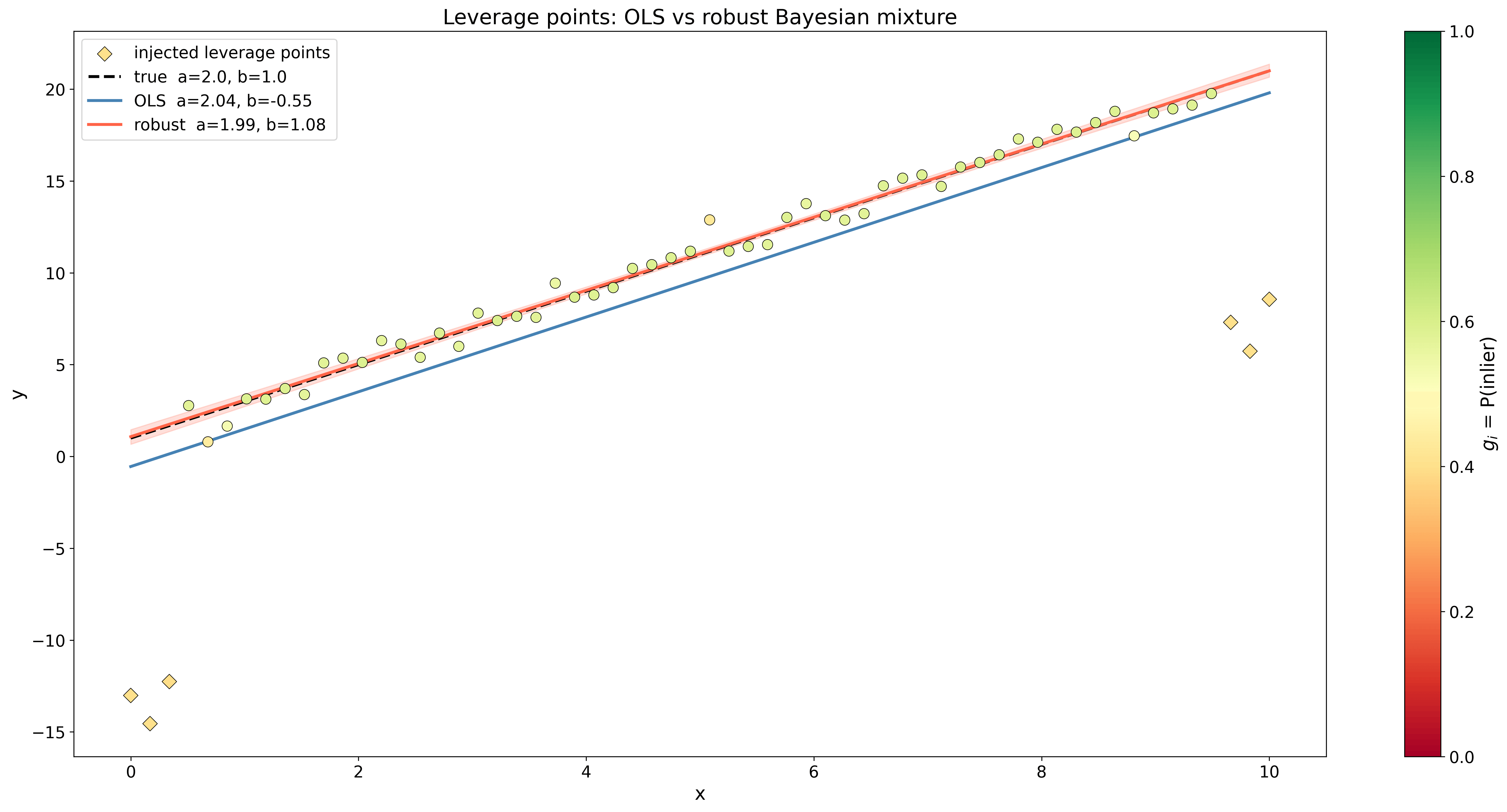
a_mean = trace.posterior["a"].values.mean()b_mean = trace.posterior["b"].values.mean()sigma_mean = trace.posterior["sigma"].values.mean()A cool perk of this approach is that it also works very well if for example your data has outliers. In this case, you can add a nuisance parameter for each data point which interpolates between our Gaussian likelihood and another Gaussian distribution with a much wider variance, modeling a background noise. This largely increases the number of unknown parameters, but in exchange every parameter is weighed and the model can easily identify outliers. In pymc, this would be done like this:
with pm.Model() as model:    # Priors    a = pm.Normal("a", mu=0, sigma=10)    b = pm.Normal("b", mu=0, sigma=10)
    # Variance of the two mixture Gaussians    sigma = pm.HalfNormal("sigma", sigma=10)    delta = pm.HalfNormal("delta", sigma=5)    sigma_bgd = pm.Deterministic("sigma_bgd", sigma + delta)    # For the background variance, ensure it's larger    # than the inlier variance by adding a positive delta.    # This helps breaking the symmetry between    # the two components and allows the model to better identify outliers.
    # Mixture weights    gs = pm.Beta("gs", alpha=2, beta=2, shape=len(x))

    # Likelihood as a weighted mixture
    mu = a * x + b    w = pm.math.stack([gs, 1 - gs], axis=1)    pm.Mixture(        "likelihood",        w=w,        comp_dists=[            pm.Normal.dist(mu=mu, sigma=v),            pm.Normal.dist(mu=mu, sigma=sigma_bgd),        ],        observed=y,    )
    # Sample from the posterior    trace = pm.sample(1000, tune=1000, chains=4)
So when is near 1, the likelihood is dominated by the regression Gaussian while when is closer to 0, the mixture tends towards the background Gaussian. In the figure below, you can see how this method compared to least-squares linear regression.
As a data scientist, you are probably used to solving problems like this using regularized linear regressions like Lasso (L1) or Ridge (L2) regressions. Under the hood, this is equivalent to finding the MAP of the parameter based on a Laplace or a Gaussian prior. If you use the log version of Bayes’ theorem with the regression likelihood, then maximizing the posterior distribution becomes a minimization
For a Gaussian prior so while for a Laplace prior , then . So all along, these two regularization techniques were just different choices of Bayesian priors!
Conclusion
I hope this post has given you some better idea of how Bayesian statistics work and where they shine. In general, I find it a better framework for fitting uncertain data and while it may sound a bit more complex, you can see from the code examples that MCMC methods make it very easy to just craft complex models from priors and data.
References
- Frequentism and Bayesianism: A Practical Introduction
- A Modern Introduction to Probabilistic Programming with PyMC
- PyMC library homepage
Footnotes
-
Right? Please tell me I’m not the only one. ↩
-
There are actually some annoying subtleties here because the distribution is discrete but the CI ends between 6 and 7, so depending on how you round you may get some coverage issue on the 95% CI. But I’m going to sweep this under the rug. ↩
-
For those interested, the behind-the-scenes for this statement is the Bernstein-von Mises theorem which essentially states that in some limit the posterior converges to a normal distribution centered around the maximum-likelihood estimation (the frequentist answer) with a shrinking width. In this same limit, the likelihood dominates the prior and completely controls the posterior, such that Bayesian and frequentist approaches agree. ↩