Forecasting energy demand using Skforecast
Last Updated:
Welcome back, everyone! In this previous post, I was talking about what topics I’d like to write about in 2025, hoping that putting my plans in writing would help me sticking with them. And so far, it’s worked! Today, I want to share an update on a project I worked on early last year and which I revisited this past week: building a forecasting pipeline to predict energy demand in France using machine learning.
Project Overview
When I first started with this project, there were specific aspects I wanted to focus on, like:
- how to work with timeseries and causal data (especially compared to a typical ML project),
- how to deal with API’s and regularly updated data,
- how to build an end-to-end MLOps pipeline, particularly automating model tuning/training and even tackling model retraining.
With these goals in mind, I set out to find a good data source and build a project structure that would satisfy all these requirements. After searching a while, I found out about Entso-e, a European platform that promotes transparency in energy production and consumption.1 This was the perfect source to work with: data related to energy demand is usually regular and seasonal, so not too difficult to predict. To narrow the scope of the project, I decided to focus solely on the French energy grid. In addition to the actual demand data, Entso-e also provides a day-ahead forecast2 which can serve as a comparison for the accuracy of my own models.
With the data source chosen, all that’s left is writing a package to pull the data from the API (on a schedule), parse it into a digestible form, then train a forecasting model on the data, and finally generate a visualization of the result. Piece of cake right?
Tour of the project
Let’s start with a diagram summarizing the interactions of the various modules of the codebase. I will go through most of them, describe how I implemented them and how they fit into the bigger picture.

CLI Interface
All the functionalities of the program are accessible through a command-line interface, built using the argparse module, in main.py. This makes it very easy to then automate behaviour in a CI/CD workflow. To use the various functions of the interface, you can simply call python main.py command,3 where command can be one of {download, merge, train, predict}.
You can provide an optional starting and end date arguments to the download command if you’d like to download a specific period, otherwise it will default to the period since the last download. The merge command merges all the fragmented timeseries into a single .csv file. It’s automatically applied during the download operation, but if you modify any of the raw files manually (or even delete some), it can be useful to call it manually.
When you call the train command, the program will create a new model and tune its hyperparameters using a portion of the dataset—this can take a couple of minutes so feel free to go grab a coffee. The model is only retrained if more than a week has passed since the end of the last training.
Finally, once the model is fully tuned and trained, the predict command will infer the timeseries value on the future (or test) part of the dataset. You can also provide the optional argument --plot to this command if you want to create a plot of the result and have it displayed on the index.html page.
This entire workflow is scheduled through Github actions, every Monday-Wednesday-Friday, using the following .yaml workflow configuration:
name: Download and Train Modelon: schedule: - cron: "0 0 * * MON,WED,FRI" # Scheduled three times a week workflow_dispatch: # Allows for manual triggeringjobs: download-tune: runs-on: ubuntu-latest steps: - name: Checkout repo content uses: actions/checkout@v4 with: token: ${{ secrets.PERSONAL_ACCESS_TOKEN }} # Use the PAT instead of the default GITHUB_TOKEN - name: Install uv uses: astral-sh/setup-uv@v5 with: # Install a specific version of uv. version: "0.5.1" enable-cache: true cache-dependency-glob: "uv.lock" - name: Setup python uses: actions/setup-python@v5 with: python-version-file: "pyproject.toml" cache: 'pip' - name: Install the project run: uv sync --all-extras --dev - name: Make envfile uses: SpicyPizza/create-envfile@v2.0 with: envkey_API_KEY: ${{ secrets.API_KEY }} # The API key is stored in the .env file file_name: .env fail_on_empty: false sort_keys: false - name: Run download # Downlaod new data run: uv run main.py download - name: Run training # Train model run: uv run main.py train - name: Make demo page # Build demo page with prediction run: uv run main.py predict --plot - name: Check for changes # create env variable indicating if any changes were made id: git-check run: | git config user.name 'github-actions' git config user.email 'github-actions@github.com' git add . git diff --staged --quiet || echo "changes=true" >> $GITHUB_ENV - name: Commit and push if changes if: env.changes == 'true' # if changes made push new data to repo run: | git pull git commit -m "downloaded new data and trained model" git pushData
The module data.py is responsible for fetching and processing the data. I initially used a custom function to query the API and parse its response. But in the few months I let the pipeline run by itself, I quickly ran into issues where the API would return unexpected responses, breaking my parser and requiring a lot of error handling. After spending a bit too much time debugging, I decided to switch to the entsoe-py Python library. It was a game-changer! This library is specifically designed to handle Entso-e’s API, so it’s better equipped to handle changes in the response or fetching errors, and in the long run, it will save me a lot of time.
The downloaded data sits inside the data/raw folder as .csv files. Ideally, a more complex project would involve some form of data versioning while the data would be stored on some external storage (like AWS or GCP). In this particular case, the timeseries consist of two float64 columns and a datetime index, with about 9k rows per year. This amounts to less than 400kB of data and doesn’t require anything too complicated.
Models
To build my models and handle predictions, I have chosen to use the Skforecast library, a scikit-learn compatible library which abstracts away a lot of the specificities of timeseries while allowing for ample configuration and customization of the models. In this project, I have made use of a lot of these features so I hope this little tour of the project can also serve as a short overview of the library. For more details about both Skforecast and generally how to work with timeseries, I whole-heartedly recommend their documentation which features an excellent introduction to forecasting, in-depth user guides, and examples of how to use the library for common use-cases. I learnt a lot from going through this documentation and I can only recommend it to you too!
Now let’s dive into the code. In the module models.py, I have created a ForecasterRecursiveModel class which wraps around the ForecasterRecursive class from Skforecast. The forecast classes from Skforecast take care of creating lag and window features during predictions, and on top of this, the ForecasterRecursive class specializes in making multi-step predictions, using each prediction as input for the next one.4 If you choose a regressor (say LGBM), you can then define your forecast as:
from lightgbm import LGBMRegressorfrom skforecast.recursive import ForecasterRecursive
forecaster = ForecasterRecursive(    regressor=LGBMRegressor(random_state=1234, n_jobs=-1, verbose=-1),    lags=12,)
The goal of the ForecasterRecursiveModel class is to automatically handle hyperparameter tuning, predictions, and backtesting of the ForecasterRecursive model.
Interlude: preprocessing and feature engineering
The module preprocessing.py contains two important classes to handle data prior to doing any training or prediction. The class LinearlyInterpolateTS helps with missing data in the downloaded timeseries. The second class, ExogBuilder, creates exogeneous features based on the index of the timeseries. I determined which calendar features to consider when exploring the data and settled with:
- a
holidaysboolean column, built using the holidays Python package, which indicates which days are French national holidays, - an
is_weekendboolean column indicating whether the day of the week in Saturday or Sunday, - multiple columns where indicates a seasonality (period) and is the order of the encoding.
This last set of features is crucial to really capture all of the seasonality for this kind of data. During the exploratory phase, I found various seasonalities in the data: energy demand generally depends on the seasonal temperature variations, the day/night cycle, and the work/weekend cycle. There are multiple ways to determine the various frequencies present in the data, like looking at autocorrelation plots or superimposing data grouped by various periodicities (for example, yearly data plotted by month, etc…). My favorite method is to use a simple Fourier analysis. Here is an example of how you can do this using scipy.signal, with a plot of the resulting spectrum:
from scipy.signal import periodogram
frequencies, spectrum = periodogram(    y, # Timeseries    window="boxcar",    scaling="spectrum",)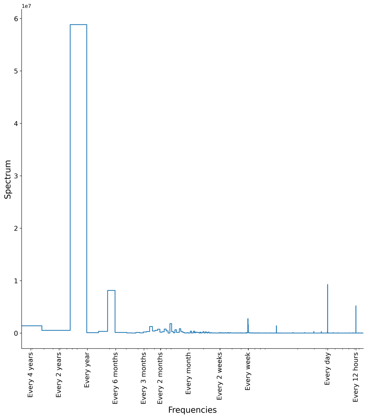
The peaks on this graph indicate the frequencies which are the most important for the data: there is a strong annual signal and slightly weaker bi-annual seasonality which match the pattern between summer and winter demand. There are also well-defined weekly and daily seasonalities, and even a twice-daily peak which is usually a sign of peak/off-peak times. Finally there is some signal in the monthly range which is less sharp, showing more variation than the others.
There are a few ways to account for these patterns in the exogeneous features, and a good summary of these is present in the Skforecast documentation. The basic idea with cyclical encoding is that, if you have a feature X[col] which you know is periodic, then you want to somehow encode that the last value is close to the first value of your period. For example, with hours, 01:00 is as close to 23:00 as it is to 03:00. Or Sunday (7) being close to both Monday (1) and Saturday (6). Ordinal encoding just doesn’t reflect that.
I have often used Fourier decompositions which can be neatly done through the statsmodels library. However, I have found better performance with the radial basis functions decomposition, which you can do with the preprocessing module of the sklego library.
With Fourier decomposition, you just replace your column by two new features: a cosine and a sine with the same period. Then your model learns from them to recognize the seasonality (daily, weekly, etc…).
Radial basis functions work the same way, except that instead of adding two new trigonometric features, you can add shifted periodic Gaussian features. In practice, this encoding seems to yield better results than Fourier modes. The number of functions added is a parameter you can choose: in this project I tended to use the periodicity itself (7 in a week, 12 in a month) if it’s small enough, or a sensible divider: 12 for the hours or 12 for the days in the year (with each function encodes the beginning of a month).
There’s another set of useful features that can be included to improve model accuracy which I mentioned before:
- lags, which are shifted versions of the timeseries itself,
- window features, which are target features calculated on a rolling window over the data.
Since both of these are based on target values, the Skforecast module handles this through the forecaster object directly. This is what the lags parameter is for in the ForecasterRecursive object, and there is a similar one for window features.
Back to model training
With the exogeneous features set, you still need to choose a model. For this type of problem, boosting-based models tend to work quite well, so I made the wrapper compatible with both XGBoost and LGBM regressors. Which one to choose is a matter of testing which one works better, and from my experiments I ended up favoring LGBM as it seemed to be overfitting less than XGBoost.5 In both cases, I included L1 and L2 regularization parameters, which help to improve the generalization of the model.
Finally, it’s time to tune the model’s hyperparameters on a cross-validation dev set before setting it in production. The tuning uses Bayesian search on an appropriate range of parameters, as well as the number of lags to include. With Skforecast, you can do hyperparameter tuning using causal cross-validation folds, i.e., separate data into folds of training and dev datasets where all the training data is before the dev data. Here is a small example of how to create these folds:
from skforecast.model_selection import TimeSeriesFold
cv = TimeSeriesFold(    steps=24, # Number of steps to predict    refit=False, # Whether to refit between each fold. If an int is given refit intermittently    initial_train_size=24*365*3, # Train over 3 years of data    allow_incomplete_fold=True, # If the last fold is not complete, still use it)
This cross-validation object can then be used when backtesting or when searching for hyperparameters. Here is an example on how to do the latter:
from skforecast.model_selection import bayesian_search_forecasterfrom optuna.trial import Trial
def search_space_lgbm(trial: Trial) -> dict:  """Function describing the search space for hyperparameters of an LGBM model."""  search_space = {      "num_leaves": trial.suggest_int("num_leaves", 8, 256),      "max_depth": trial.suggest_int("max_depth", 3, 16),      "learning_rate": trial.suggest_float("learning_rate", 0.001, 0.2, log=True),      "n_estimators": trial.suggest_int("n_estimators", 50, 1000, log=True),      "bagging_fraction": trial.suggest_float("bagging_fraction", 0.5, 1),      "feature_fraction": trial.suggest_float("feature_fraction", 0.5, 1),      "reg_alpha": trial.suggest_float("reg_alpha", 0.01, 100),      "reg_lambda": trial.suggest_float("reg_lambda", 0.01, 100),      "lags": trial.suggest_categorical("lags", c.lags_consider),  }  return search_space
# The Bayesian search forecaster uses Optunaresults, _ = bayesian_search_forecaster(    forecaster=forecaster, # The forecaster object    y=y, # Timeseries data of shape (N,1)    cv=cv, # The cross-validation folds    search_space=search_space_lgbm, # Range of parameters to consider    metric="mean_absolute_error",    exog=X, # Exogeneous features of shape (N, n_features)    return_best=False, # If True, the model will be retrained on the best parameters found    random_state=c.random_state,    verbose=False,    n_trials=10, # Number of trials to find the right parameters)
print(f"Best parameters:\n {results.iloc[0]}")
There are various strategies you can choose from in cross-validation: whether you want to refit the regressor between each fold, intermittently, or never, but also whether you want to keep the training size fixed, etc… The preceding example only showed a sample of what’s possible, and I recommend going through the Skforecast documentation for more details.
My advice is to always choose a strategy that resembles as much as possible the actual prediction scenario. In my case, the program will predict batches of 24 hours of data, with retraining every 7 days, so I chose to work with a fold size of 24, and the model should be refitted every 7 folds. However, to reduce the computational load, I also chose not to refit the model during cross-validation, even though it would be more accurate: sometimes you have to make some compromises for performance!
Once the model is tuned, the ForecasterRecursiveModel class is then fitted on the whole training + dev sets of data before making new predictions. Finally, the model is serialized to a file using the dill library, so it can be easily loaded when it’s time to make inferences. I initially used joblib for this part, but after refactoring the code, it somehow stopped working. I couldn’t find the exact reason why the joblib library suddenly failed, but as usual the dill library worked when joblib wouldn’t. However, this isn’t a complete fix to me, and an improved version of this function would be to save only the regressor instead of dumping the whole ForecasterRecursiveLGBM object.
Results
So what does it look like in the end? Well here is a sample of the kind of output this code generates, and a live demo is accessible here.
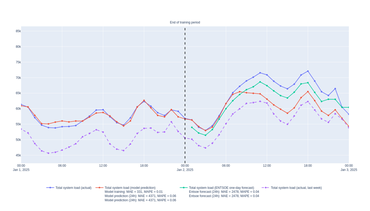
Hurray! The error on the prediction is small and seems quite close to the black box forecast Entso-e provides. Note that in the live demo, this can vary depending on the latest training and what the data looks like at the moment. In any case, this is great news as this was a simple implementation, and it yielded results on par or close to the reference forecast from the data source.
Feature importance: Can we say anything more about this model?
An important part of any ML project is explainability: it’s all good and well to make predictive models, but it’s important to be able to explain how your model works and why it’s making some predictions. Thankfully, the shap library comes to the rescue! Based on game theory,6 this library brings a simple way to evaluate which feature matters the most to make predictions. In the case of an LGBM model trained over the last 3 years, these are the top features in terms of averaged shap values:
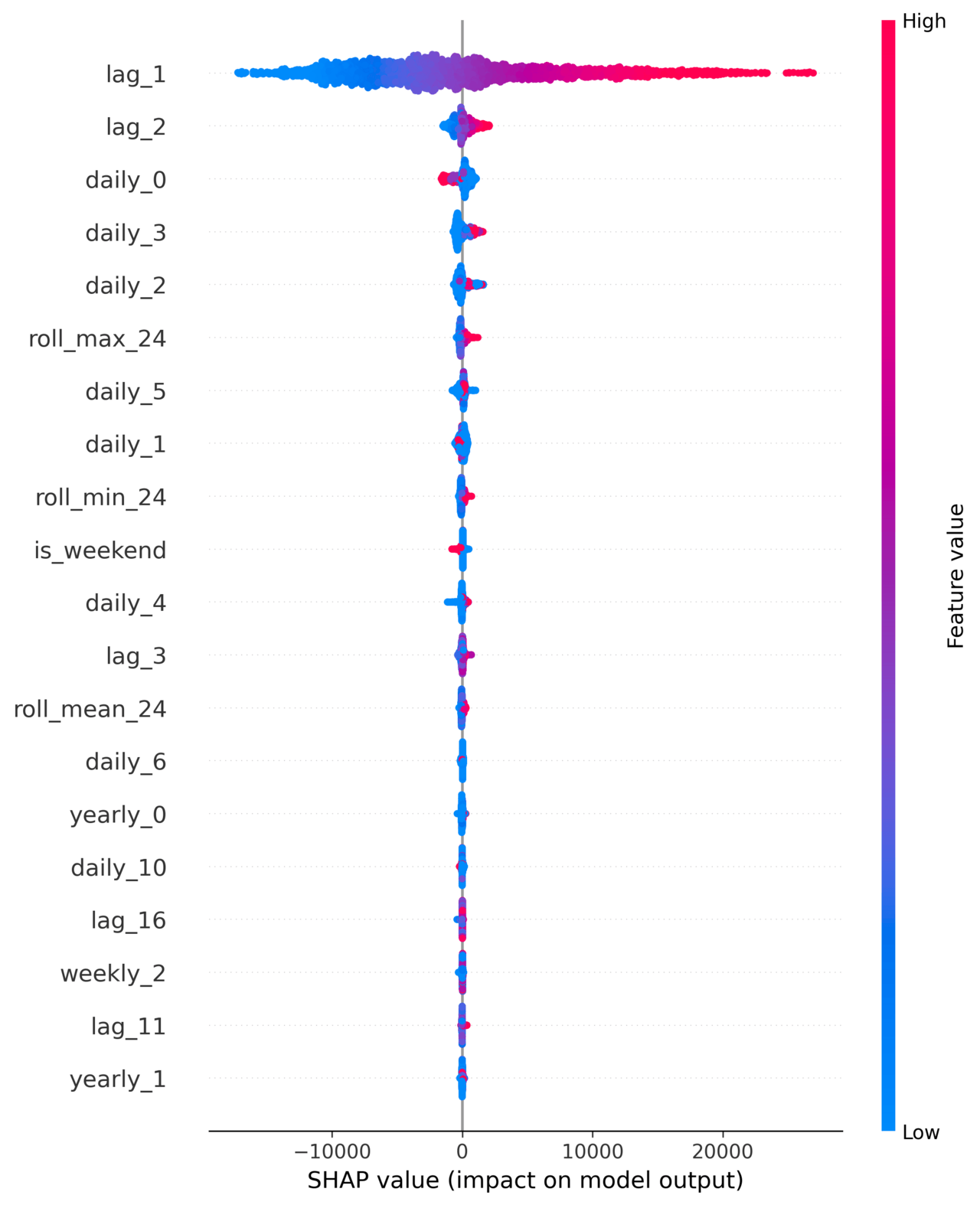
Let’s take a closer look at this plot and figure out why each of these features contribute to the model in this way:
- the first lag: this is usually an important feature of timeseries as the next time step tends to be strongly correlated to the current time step.
- The daily, weekly and yearly cyclical features. As I’ve mentioned before, energy demand tends to trend strongly with seasons and with daily usage so it’s not surprising to see these features matter a lot here.
- Rolling window features: these features tend to average seasonal effects and instead encode for evolving trends.
- Other lag features: most timeseries tend to depend on higher-order lag features. Putting my physicist cap on, a timeseries which would only depend on the first lag would most likely be some exponentially damped system,7 while a second-order lag dependency would be reminiscent of periodic systems, like harmonic oscillators. More complicated systems will either involve more complex couplings or higher-order dependencies.
Since I am using LGBM as a regressor, I can also peek into the output of its native get_feature_importance() method and see the top 10 most important features:
| feature | importance |
|---|---|
| lag_1 | 3675 |
| daily_0 | 2839 |
| yearly_0 | 2147 |
| lag_3 | 1922 |
| lag_2 | 1872 |
| daily_2 | 1819 |
| daily_4 | 1808 |
| roll_mean_168 | 1460 |
| daily_1 | 1450 |
| roll_min_24 | 1420 |
While the exact number itself isn’t that important, the order and relative magnitude gives an idea as to which features matter most. It’s a good sign that this list agrees with the SHAP summary plot and tells the same story.
Revisiting the project: key lessons
One of the most interesting takeaways from this project was how tough it can be to improve upon an existing project. There’s a fine line between over-engineering a codebase by trying to foresee future refactoring that won’t happen, and accumulating technical debt by not writing maintainable and extendable code. I personally tend to fall on the side of the former, creating more and more abstraction than is generally needed. Surprisingly when I came back to this codebase, I realized I was instead fighting with most of the decisions I had made early on.
This experience also reaffirmed something I had learnt before: it’s easy to think that improving a project means adding new features, but it’s just as important to take a step back and simplify things. After refactoring the code, I realized that simplifying the structure and focusing on the essentials helped me achieve better results with less complexity.
Conclusion
This project was very rewarding: I learnt some hard lessons (for example, use a library to handle your API if you can), how to structure an ML training pipeline, and even how to troubleshoot serialization issues in GitHub Actions.
As I continue to build on this project and refine it, I’m really looking forward to exploring further ways to improve and extend it, especially now that I have a clearer understanding of what works (and what doesn’t). Hopefully, this post was helpful for anyone looking to build their own forecasting pipelines, or anyone just generally interested in timeseries forecasting, and I look forward to sharing more lessons and projects in the future!
Stay tuned for more updates, and feel free to reach out with any questions or feedback!
Footnotes
-
To get access to the API, you first need to email the support with some motivation as to why you need it. They’re very responsive and happy to share their API for educational purposes. ↩
-
Unfortunately, I found no documentation on how they made this forecast and what the methodology employed is. ↩
-
I have recently been using the uv Python package manager and it’s been a blast! It can handle python versions, virtual environments, and it happens to be super fast. With it, you can quickly install the project with
uv sync. Calling the program then requires to go throughuvwithuv run main.py command. ↩ -
The Skforecast library also features the class
ForecasterDirectwhich, instead of recursively using the predictions as input, trains as many models as prediction points. Which one to choose is up to you: the recursive method will compound errors while the direct method can be quite resource intensive given the number of models to train, and tends to treat predictions independently. ↩ -
Interestingly, I recently had the complete opposite experience with another dataset, where XGBoost consistently outperformed LGBM. This is a good reminder that there is rarely a one-size-fits-all model and tests should drive your choices. ↩
-
The basic idea behind SHAP values is to consider a competition between features and see which ones are most important to go from the average predicted value of the target to a given prediction. This is a popular way to measure the relative importance of each feature, both locally and globally. ↩
-
And it could likely be approximated with exponential smoothing average. ↩