Ising model, Metropolis sampling and genetic algorithms

15 Sept 2024

34 min read

Introduction

Welcome to the first deep dive of this blog! Following my initial post, I’m excited to explore a physics-based project which I found particularly engaging: solving the Ising model with genetic algorithms.

Animation of spins

I became fascinated by genetic algorithms the moment I first heard of them. The simple concept of treating a problem to solve like some constraint on a population immediately hooked me. As a good physicist, I had to find a way to play with these in my natural habitat. I remembered from my university days that the Ising model was easy enough to solve, and I thought it wouldn’t hurt to dust off my knowledge of Monte Carlo methods—which are traditionally used for this problem. And so here we are!

This post is a good example of the kind of technical physics I want to write about, while remaining generally accessible. I marked the advanced sections which might require more physics knowledge for those curious to learn more about it. If that’s not you, don’t worry! You can just skip them and move to the code part!

Physics background: the Ising model

Let’s begin with an introduction of the Ising model¹, one of the most widely studied models in physics. Despite its apparent simplicity, the Ising model showcases some interesting physical phenomena such as phase transitions and Renormalization, which are to this day active research topics. This is going to be a physics-heavy section, so let’s get to it!

At its core, the Ising model represents a magnet as an organized collection (or lattice) of atoms. Each site in this lattice contains an arrow (or spin) pointing either up or down, indicating the direction of local magnetization. When all arrows align in the same direction, you have a ferromagnet, which produces a magnetic field in that direction—the same as the magnets on your fridge! On the other hand, when the arrows point randomly in different directions, the overall magnetization is zero, resulting in a paramagnet. The system then behaves like an ordinary piece of metal until you place it in an external magnetic field.

To summarize: a ferromagnet possesses inherent magnetism, while a paramagnet only responds to external sources of magnetism. There’s also a third interesting case called anti-ferromagnets, where each arrow points in the opposite direction to its neighbors, creating a pattern resembling a checkerboard. Anti-ferromagnets are interesting because they produce good electronic insulators, for example Mott insulators.

Detailed section

If this small introduction has caught your interest, here are now some more details. The Ising model goes beyond just describing spin directions; it also defines how these spins interact with each other and their environment. Three important energy scales determine the system’s behavior:

The energy $J_0$ gained from two neighboring spins being aligned.
The energy $h_0$ gained from a spin aligning with an external magnetic field.
The thermal energy scale $k_B T$ .

You can summarize these interactions in a mathematical object called a Hamiltonian:

H = -J_0 \sum_{\langle i,j \rangle} s_i s_j -h_0 \sum_i s_i~.

In particular, if you evaluate the Hamiltonian on some configuration, it will be equal to the energy of the system.

NOTE

The symbol $\sum_{\langle i,j \rangle}$ means a summation over all nearest-neighbor pairs of sites $i,j$ .

For a given configuration of spins $\{s_i\}$ at some temperature $T$ , the probability $P(\{s_i\})$ of the system to be in that configuration obeys the Boltzmann distribution. This means that $P(\{s_i\}) = \frac{e^{- H(\{s_i\})/k_B T}}{\sum_{\{s_j\}} e^{- H(\{s_j\})/k_B T}}$ . The denominator of this expression is also named the partition function $Z$ and is there to normalize the probability distribution.

You can also work with the rescaled Hamiltonian $\hat H = \frac{H}{k_B T}$ along with rescaled parameters $J = \frac{J_0}{k_B T}$ and $h = \frac{h_0}{k_B T}$ . Doing so helps seeing how each term influences the system’s behavior:

When $h>0$ dominates, the system tends to align with the external field.
When $J>0$ dominates, the spins tend to align with each other, resulting in a ferromagnetic phase. A negative $J$ leads to an anti-ferromagnetic phase.
When both terms are relatively small, temperature fluctuations govern the system’s dynamics, resulting in a paramagnetic phase.

CAUTION

Physicists often work with the inverse temperature parameter $\beta = \frac{1}{k_B T}$ . This is the convention I’ll use in the code for this project.

Finally, the Ising model has an exactly known solution in two dimensions.² This is great news, it tells us at which temperature (or coupling) the transition happens! In terms of the dimensionless variable $J = \frac{J_0}{k_B T}$ (and when $h = 0$ ), the critical coupling is $J_c = \log (1 + \sqrt{2})/2$ and the average magnetization below the critical temperature is $M = \bigl[ 1 - \sinh(2 J)^{-4} \bigr]^{1/8}$ . This will be useful when I compare the numerical data to the theory.

Why is this such an interesting model?

After all these details, let’s see why physicists love this model. Its main feature is the phase transition between the paramagnetic and ferromagnetic states. As the system cools down, it eventually reaches the critical Curie temperature, at which point the spins spontaneously align. This is what distinguishes ferromagnets from paramagnets in real life: both materials behave like paramagnets at high temperatures, but only ferromagnets undergo this transition at lower temperatures. To put things in perspective, the Curie temperature of iron is 770°C which can be reached with a simple candle!

Interestingly, even without an external magnetic field, the system will select one of the two possible alignments when it cools down. This phenomenon, known as spontaneous symmetry breaking, is an important concept in physics. In fact, it also plays a big role in the behaviour of subatomic particles, such as the Higgs boson discovered in 2012.

If it seems complicated, maybe this analogy will help: if you put a pen perfectly straight up on a table, it will eventually fall on its side. If the pen is perfectly balanced, how does it choose which side to fall on? Mathematically, the angle at which it falls is spontaneously chosen the moment you let it go. Of course, this concept really only works in the ideal world of mathematics. In the real world, there are all sorts of small effects which determine where the pen will fall. For example, never being perfectly balanced, the motion you make when you let it go, whether there is some air current in the room, etc…

Another significant aspect of the Ising model is that its phase transition defines a universality class. This concept means that different systems can exhibit similar physics near a phase transition, regardless of their specific composition. For instance, the Ising model also describes the transition between a liquid and a gas on a lattice, where the density of molecules plays the role of the spins. This is surprising considering spins and water molecules have little to do with each other. The reason for this is that the system breaks the same symmetry in the same way in both cases. Therefore, by studying the Ising model, you can get insights into a wide range of physical systems beyond simple magnets.

Solving the dynamics of the Ising model

As the title of this post suggests, this deep dive is about physics and numerical simulations. So far, I have only talked about physics, that means now is the time to get coding. So get comfy and let’s dive in!

Numerical Ising configuration

To begin the numerical exploration of the Ising model, I first need to set up a representation that the computer can work with. A two-dimensional Ising configuration with $N = n^2$ spins is stored as a numpy array of shape (n,n) with values +1 (spin up) or -1 (spin down).

Both algorithms I will use require an initial configuration as input. This can be either random (mimicking a high-temperature state) or ordered (representing a low-temperature state). Let’s take a look at the code that sets this up:

import numpy as np
import numpy.random as rand
from numba import float64, int64, njit, void

@njit([int64[:, :](int64)])
def create_random_state(n):
    """Returns a random matrix of spins up and down

    Args:
        n (int): Size of the matrix

    Returns:
        np.ndarray: Matrix of shape (n,n) and random values in +1/-1.
    """
    return 2 * rand.randint(0, 2, (n, n)) - 1

@njit([int64[:, :](int64, int64)])
def create_lattice(n, state=0):
    """Creates a numpy lattice of N spins.

    Args:
        n (int): Number of spins in one dimension (total spins N = n^2).
        state (int, optional): Defines the initial state. Accepted values are 0 (hot, random state) or +1/-1 (all up, down resp.). Defaults to 0.

    Returns:
        ndarray: Numpy ndarray of spins (+1 or -1 at every site) with shape (n,n).
    """
    match state:
        case 1:
            return np.ones((n, n), dtype=np.int64)
        case -1:
            return -1 * np.ones((n, n), dtype=np.int64)
        case _:
            return create_random_state(n)

This code creates the initial lattice configuration. The function create_lattice generates a configuration with all spins up, all down, or in a random state (using create_random_state). The next step is for the algorithm to keep track of two important quantities: the energy of the system (that’s where the Hamiltonian comes in) and the average magnetization (which helps distinguishing between phases). Here’s how I compute these:

@njit([float64(int64, int64, int64[:, :])])
def compute_hamiltonian_term(x: int, y: int, lattice: np.ndarray):
    """Computes the Hamiltonian at a lattice site i,j given a lattice state as well as parameters values.

    Args:
        x (int): row of lattice site
        y (int): column of lattice site
        lattice (ndarray): lattice of spins in a given state.

    Returns:
        float64: Value of the Hamiltonian at site i,j for this configuration.
    """
    n = lattice.shape[0]
    si = lattice[x, y]
    neighbors = [((x + 1) % n, y), ((x - 1) % n, y), (x, (y + 1) % n), (x, (y - 1) % n)]
    term_sum_neighbors = np.float64(0.0)
    for neighbor in neighbors:
        term_sum_neighbors += si * lattice[neighbor]
    # Remove the extra factor of 2 due to duplicate counting of pairs
    Hi = -term_sum_neighbors / 2
    return Hi

@njit([float64(int64[:, :], float64)])
def compute_hamiltonian_from_site(lattice: np.ndarray, h: np.float64):
    """Computes the Hamiltonian given a lattice state as well as parameters values using the site method.

    Args:
        lattice (ndarray): lattice of spins in a given state.
        h (float64): External field coupling.

    Returns:
        float64: Value of the Hamiltonian for this configuration.
    """
    n = lattice.shape[0]
    H = np.float64(0.0)
    for x in range(n):
        for y in range(n):
            H += compute_hamiltonian_term(x, y, lattice)
    return H - h * np.sum(lattice)

@njit([float64(int64[:, :])])
def compute_magnetization(lattice: np.ndarray):
    """Computes the magnetization for a given lattice configuration

    Args:
        lattice (ndarray): Configuration of up and down spins

    Returns:
        float: Average magnetization of the configuration
    """
    N = np.int64(lattice.size)
    return np.sum(lattice) / N

Monte Carlo method with Metropolis sampling

Let’s begin with the traditional Monte Carlo method, which will serve as a benchmark for solving this problem.

Method overview

The Monte Carlo method is based on random sampling of configurations over a large number of steps until the statistics of the sample converge to the true underlying solution. This approach effectively mimics natural processes and is particularly useful in statistical physics.

Detailed section

When you study physics, you generally start from classical physics such as the motion of a pendulum or Newton’s laws of motion. These are purely deterministic: if you know your system well at any moment, you can predict its state at any later time.

Most people are also familiar with the idea that with quantum physics, all of this goes out the window. This theory tells us that the universe, at its fundamental level, isn’t deterministic but probabilistic, and that one can’t know the exact state of a quantum system without uncertainty. While the Ising model is easily generalizable to a quantum system, I will not be doing any quantum physics here so you can rest easy!

Statistical physics, on the other hand, allows physicists to handle systems (deterministic or not) with many interacting components by considering probabilities of states rather than tracking each component individually. This probabilistic approach is especially useful for systems like the Ising model, where the collective behavior is of more interest than individual spin states.

The Metropolis sampling algorithm, which forms the core of the Monte Carlo method, is a special way to explore the configurations of the Ising model. It can be summarized as follows:

Start with an initial configuration.
Repeat for $M$ $M$ steps:
1. Pick a random spin and flip it.
2. Calculate the energy difference $\Delta H$ $Δ H$ :
  - If $\Delta H < 0$ , accept the spin flip.
  - If $\Delta H >= 0$ , accept the flip with probability $p = e^{- \Delta H/k_B T}$ .
Compute the summary statistics of the last $M^\prime$ configurations.

This algorithm effectively minimizes the system’s energy (optimization) while allowing for some unfavorable spin flips (exploration). When the temperature is high, the probability $p$ tends to be rather large and spin flips are accepted regardless of whether they lead to a smaller or larger energy. The competition between energy minimization and temperature-driven randomness—quantified by a quantity called entropy—is a key feature of statistical physics.

Now, let’s implement this sampling algorithm step by step. I have already covered the initial configuration part in the previous section. The next two functions calculate the energy cost and magnetization change from flipping a specific spin. This way is simpler than just re-computing the entire energy of the new state.

@njit(
    [float64(int64, int64, int64[:, :], float64)],
)
def compute_deltaH(x, y, lattice: np.ndarray, h: np.float64):
    """Compute the variation of the Hamiltonian given a spin flip

    Args:
        x (int): Index of spin to flip (row)
        y (int): Index of spin to flip (column)
        lattice (np.ndarray): Spin configuration
        h (float): External coupling

    Returns:
        float: Hamiltonian change
    """
    n = lattice.shape[0]
    si = lattice[x, y]
    neighbors = [((x + 1) % n, y), ((x - 1) % n, y), (x, (y + 1) % n), (x, (y - 1) % n)]
    sum_nn = sum([lattice[nn] for nn in neighbors])
    deltaH = (-2) * (-(si) * sum_nn - si * h)
    return deltaH

@njit(
    [float64(int64, int64, int64[:, :])],
)
def compute_deltaM(x: int, y: int, lattice: np.ndarray):
    """Compute the variation of the magnetization given a spin flip

    Args:
        x (int): Index of spin to flip (row)
        y (int): Index of spin to flip (column)
        lattice (np.ndarray): Spin configuration

    Returns:
        float: Magnetization change
    """
    N = lattice.size
    return -2 * lattice[x, y] / N

All these functions then go inside the update_lattice function, which implements the core of the Metropolis algorithm:

@njit(
    [void(int64, int64, int64[:, :], float64[:], float64[:], int64, int64, float64, float64)],
)
def update_lattice(
    x: int,
    y: int,
    lattice: np.ndarray,
    energies: list,
    magnetizations: list,
    i: int,
    n: int,
    beta: np.float64,
    h: np.float64,
):
    """Update step for the Metropolic MC algorithm (in-place)

    Args:
        x (int): Index of spin to flip (row)
        y (int): Index of spin to flip (column)
        lattice (ndarray): List of lattices to update
        energies (list): List of energies to update
        magnetizations (list): List of magnetizations to update
        i (int): index of current iteration
        n (int): Length of the square lattice
        h (float): External coupling
    """
    # Since the initial state is manually set, we make here a rule to trivially exit
    if i == 0:
        return None
    # Compute the new energy and the energy difference
    deltaH = compute_deltaH(x, y, lattice, h)
    energy_flipped = energies[i - 1] + deltaH
    mag_flipped = magnetizations[i - 1] + compute_deltaM(x, y, lattice)

    # We now decide whether to accept the change or not
    accept = True
    if deltaH > 0:
        # If the energy variation is positive, we only accept under a probability threshold given by Boltzmannian weight
        probability_threshold = np.exp(-beta * deltaH)
        accept = rand.rand() < probability_threshold

    # If accepted, we flip the sign
    if accept:
        lattice[x, y] *= -1
        magnetizations[i] = mag_flipped
        energies[i] = energy_flipped
    else:
        magnetizations[i] = magnetizations[i - 1]
        energies[i] = energies[i - 1]

You can notice that this update function needs some arrays to store the properties of the new state. This is handled by the monte_carlo_metropolis function which is also in charge of looping over the Monte Carlo time steps:

def monte_carlo_metropolis(
    n: int, beta: float, h: float, max_steps=100, initial_state=0, method="checkerboard", store_history=False
):
    """General Monte Carlo simulation of Ising spins for a given number of spins, inverse temperature, spin coupling and external coupling.

    Args:
        n (int): Number of spins in one dimension (total spins N = n^2).
        beta (float): Inverse temperature.
        h (float): External field coupling.
        max_steps (int): Maximal number of updates (in volume size units). Defaults to 1000.
        initial_state (int, optional): Defines the initial state. Accepted values are 0 (hot, random state) or +1/-1. Defaults to 0.
        method (str, optional): Method to use ("random", "checkerboard"). Defaults to checkerboard.

    Returns:
        dict: Dictionary containing a list of spin configuration and observables, as well as input parameters.
        Keys are "lattices", "energies", "magnetizations", "n", "J", "beta", "h", "max_steps".
    """
    allowed_methods = ["random", "checkerboard"]
    if method not in allowed_methods:
        raise ValueError(f"Unknown method! Allowed values are: {allowed_methods}")
    if method == "checkerboard" and (n % 2) == 1:
        raise ValueError("The length of the lattice in checkerboard method should be an even integer!")
    # Convert inputs into numpy floats
    h64 = np.float64(h)
    beta64 = np.float64(beta)
    # Define method specific variables
    match method:
        case "random":
            loop_steps = max_steps * n**2 + 1
        case "checkerboard":
            loop_steps = 2 * max_steps + 1
            mask_even, mask_odd = get_mask_even(n), get_mask_odd(n)
    # Store outputs of the program
    energies = np.zeros(loop_steps, dtype=np.float64)
    magnetizations = np.zeros(loop_steps, dtype=np.float64)
    lattice_history = np.zeros((loop_steps, n, n))

    # We start by initializing the lattice
    lattice_init = create_lattice(n, state=initial_state)
    lattice = lattice_init.copy()
    lattice_history[0] = lattice_init.copy()
    energies[0] = compute_hamiltonian_from_site(lattice, h64)
    magnetizations[0] = compute_magnetization(lattice)

    for i in range(1, loop_steps):
        match method:
            case "random":
                random_method(i, lattice, beta64, h64, energies, magnetizations)
            case "checkerboard":
                checkerboard(i, lattice, beta64, h64, energies, magnetizations, mask_even, mask_odd)
        if store_history:
            lattice_history[i] = lattice.copy()

    benergies = [beta64 * energy for energy in energies]

    object_return = {
        "lattice": lattice,
        "lattice_init": lattice_init,
        "benergies": benergies,
        "magnetizations": magnetizations,
        "energy_per_site": energies / n**2,
        "n": n,
        "beta": beta64,
        "h": h64,
        "number_steps": loop_steps,
        "time": np.arange(1, loop_steps + 1),
        "lattice_history": lattice_history,
    }

    return object_return

You probably noticed that this function can handle various solving methods (defined by the variable allowed_methods) which I have not really defined so far. There are a few possible choices for the function used to determine which spin to flip, and I will now go over them.

Selection method

In its basic formulation, the Metropolis algorithm just indicates to choose random spins to flip one after another, which is what the random method in the code does, using the following selection function

@njit([void(int64, int64[:, :], float64, float64, float64[:], float64[:])])
def random_method(i, lattice, beta64, h64, energies, magnetizations):
    """This method picks a random spin N = n^2 times and updates the lattice.

    Args:
        i (int): Index of Monte-Carlo step.
        lattice (np.ndarray): List of lattices to update.
        beta64 (np.float64): Inverse temperature.
        h64 (np.float64): External coupling.
        energies (np.ndarray): History of energies.
        magnetizations (np.ndarray): History of magnetizations.
    """
    n = lattice.shape[0]
    x, y = (int(rand.rand() * n), int(rand.rand() * n))
    update_lattice(x, y, lattice, energies, magnetizations, i, n, beta64, h64)

However, you might remember that the Hamiltonian of the Ising model only involves nearest-neighbor spins. So if you take two spins which are not neighbors, they’re not interacting! This opens up a great way to speed up the convergence of the Monte-Carlo exploration process: you can flip half of all the spins at the same time, independently, if you pick them in a checkerboard pattern: .

This method is generally faster and more effective than looping over random choices. Still, after a long number of iterations, both should land on the same solution. To implement this method, I used two helper functions to define the checkerboard masks:

@njit([int64[:, :](int64)])
def get_mask_even(n):
    """Returns an (n,n) matrix filled with 0,1 in a checkerboard pattern (0 on top-left cell)

    Args:
        n (int): Shape of matrix
    Returns:
        np.ndarray: Mask matrix
    """
    mask_basic = np.indices((n, n)).sum(axis=0) % 2
    return mask_basic


@njit([int64[:, :](int64)])
def get_mask_odd(n):
    """Returns an (n,n) matrix filled with 0,1 in a checkerboard pattern (1 on top-left cell)

    Args:
        n (int): Shape of matrix
    Returns:
        np.ndarray: Mask matrix
    """
    mask_basic = np.indices((n, n)).sum(axis=0) % 2
    return 1 - mask_basic

The checkerboard method then simply alternates the spin flip procedure on each half-lattice mask. To optimize the computation further, I used the np.roll function to quickly calculate the nearest-neighbor Hamiltonian term. Unfortunately, at the time of writing of this post, Numba doesn’t handle this matrix operation. Surprisingly, the trade-off from not using Just In Time (JIT) compilation on this function was worth it.

def checkerboard(i, lattice, beta64, h64, energies, magnetizations, mask_even, mask_odd):
    """This method updates the N spins in two batches of N/2 in a checkerboard pattern allowing for parallelization.

    Args:
        i (int): Index of Monte-Carlo step.
        lattice (np.ndarray): List of lattices to update.
        beta64 (np.float64): Inverse temperature.
        h64 (np.float64): External coupling.
        energies (np.ndarray): History of energies.
        magnetizations (np.ndarray): History of magnetizations.
    """
    # We extract the checkerboard sublattice matching the parity of the iteration counter
    n = lattice.shape[0]
    sublattice = (i - 1) % 2
    mask = mask_even if sublattice == 0 else mask_odd
    # We compute the energy and magnetization variations for each spin flips
    sum_nn_terms = (
        np.roll(lattice, 1, axis=0)
        + np.roll(lattice, -1, axis=0)
        + np.roll(lattice, 1, axis=1)
        + np.roll(lattice, -1, axis=1)
    )
    neighbour_contributions = -lattice * (sum_nn_terms) - h64 * lattice
    delta_contributions_flipped = -2 * neighbour_contributions
    mag_flipped = -2 * lattice / n**2

    # Generate random flips and compare to boltzmann weights
    random_flips = rand.rand(n, n)
    boltzmann_weights = np.exp(-beta64 * delta_contributions_flipped)
    random_mask = random_flips < boltzmann_weights

    accepted_flips = mask * ((delta_contributions_flipped < 0) | ((delta_contributions_flipped > 0) & random_mask))

    lattice *= 1 - 2 * accepted_flips
    magnetizations[i] = magnetizations[i - 1] + np.sum(mag_flipped * accepted_flips)
    energies[i] = energies[i - 1] + np.sum(delta_contributions_flipped * accepted_flips)

Results

This has been a lot of preparation, and now it’s time to see what the simulation says! The Monte Carlo algorithm mimics real temperature fluctuations until the system reaches its equilibrium configuration. To illustrate this, let’s examine two contrasting scenarios:

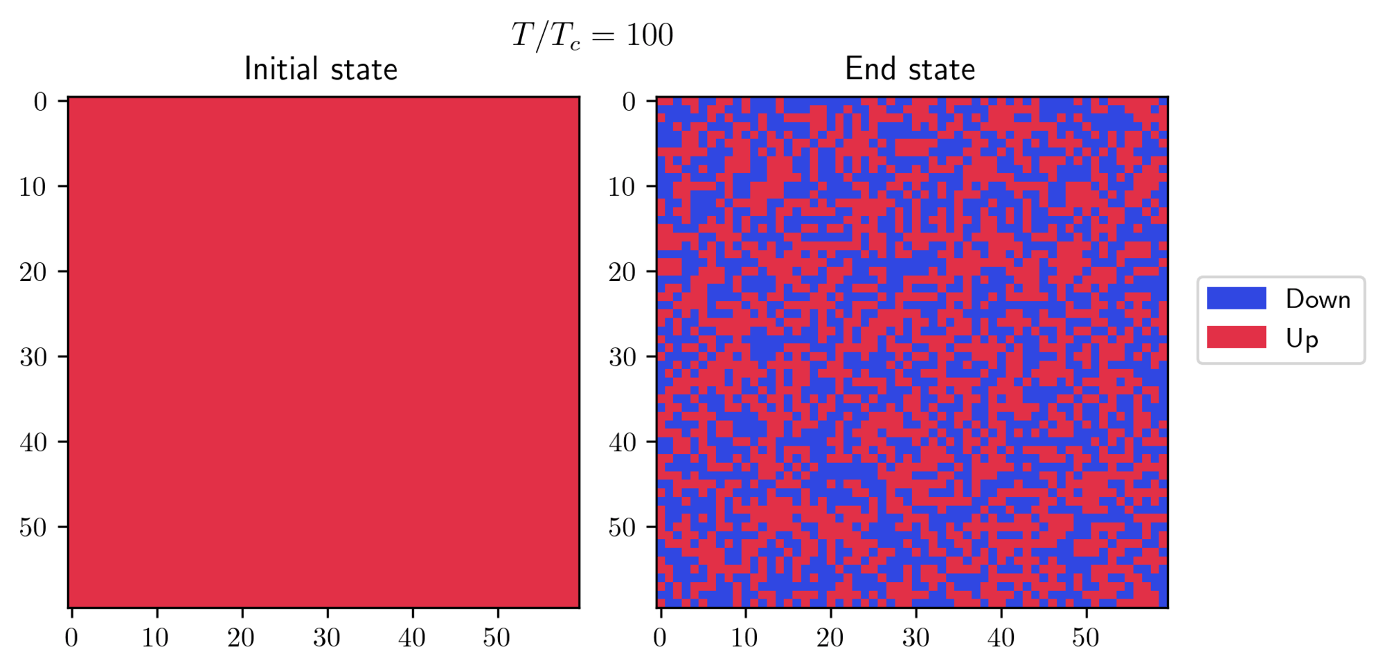
First, I initialized the system in a “cold” state, where all spins are aligned, and then I exposed it to a high temperature. I let the algorithm run for approximately 200 steps and this is what I obtained:
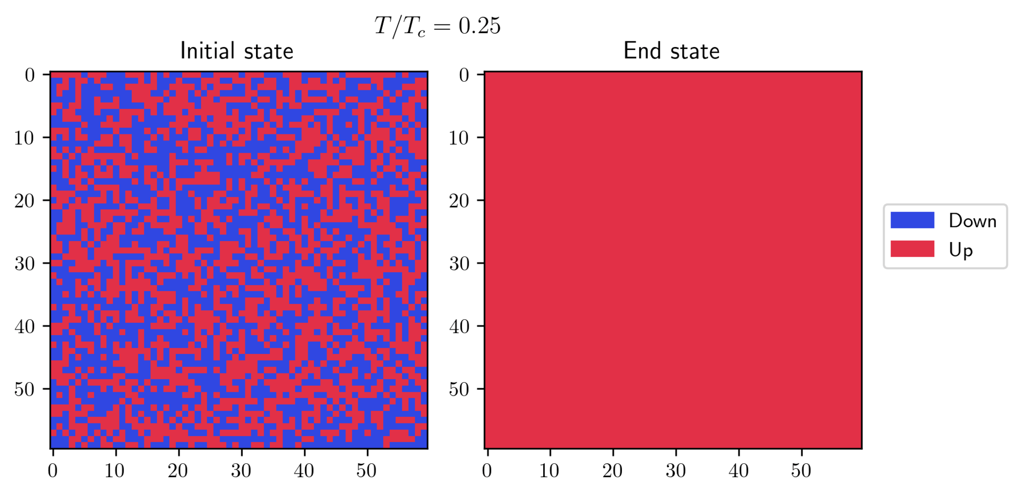
On the other hand, I started with a “hot” initial state and observed how it behaves at a lower temperature. There’s a small trick required to achieve this result: you need to set a small value for the external field h = 0.005, but not zero. This little push is necessary to help the system pick one of the two possible solutions at this temperature. In both cases, the systems eventually found its true equilibrium state! There’s another interesting effect which can be seen at or near the transition temperature:

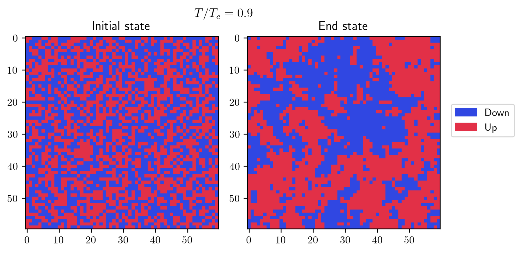
Near the critical point, the fluctuations are strong, preventing the system from settling into a uniform state. Instead, you can see the formation of patches with different spin orientations. The size of these patches is characterized by a crucial parameter known as the correlation length. This length grows dramatically as the temperature approaches the transition temperature, theoretically becoming infinite at the exact transition point.

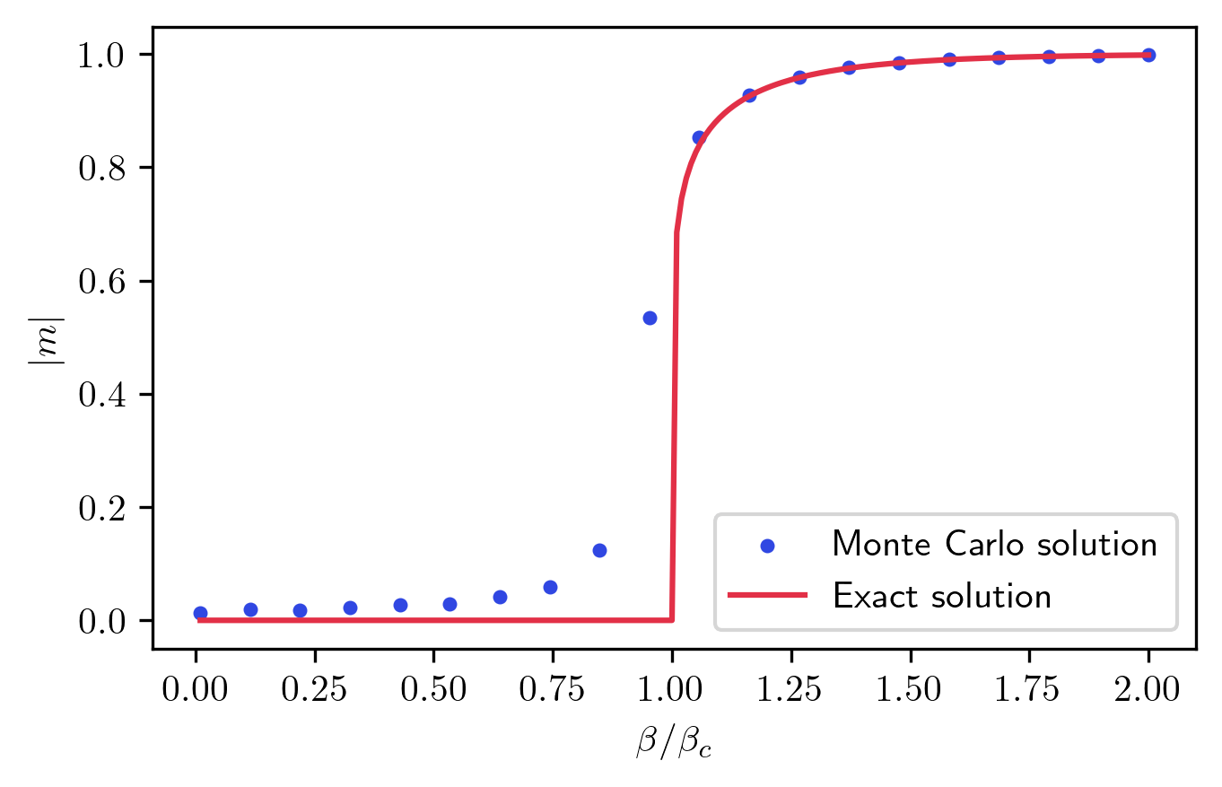
So far, the numerical solution behaves as expected, but this can be taken further. Since the 2D Ising model has an exact analytical solution, I can directly compare it with the numerical results: Comparison magnetization to exact solution

The magnetization curve from the numerical data matches well with the analytical formula! There’s however a slight discrepancy near the transition point. This is due to the large correlation length in that region. To achieve higher accuracy, I would need to extend the Monte Carlo sampling over a longer period.

After all this effort, the method works! In the next section, I will follow the same path as I build the genetic algorithm.

Genetic algorithms

Method

Genetic algorithms are a class of methods to solve optimization problems. These are problems where you need to find the maximum or minimum of some unknown function $f(x)$ , called the objective function. With genetic algorithms, you can estimate the optimal solution by mimicking the process of natural section in the theory of evolution. The basic idea is to create a population of possible solutions, characterized by properties called genes by analogy. Starting from this population, one then needs to loop over three steps: reproduction, mutation, and selection. The various loop iterations are like successive generations and the reproduction part just means creating new solution elements (called children) from members of the population (the parents). The mutation part of the algorithm is essential: it allows to keep some genetic diversity in the solutions. Finally, you should rank all members of the population using the objective function, and drop the least-fit members before moving to the new generation. In pseudocode, the algorithm would look like this:

Initialization: start from a random population of $N$ members.
Evolution: repeat these steps over $M$ $M$ generations
1. Pick $N^\prime$ $N^{'}$ random pairs of parents to generate $P$ $P$ children:
  - Each child inherits some of the genes from their parents.
  - The genes of each child are randomly mutated.
2. All $N + P \times N^\prime$ members of the population are then evaluated by the objective function and ranked.
3. Only the top $N$ members survive the selection process.

After a sufficiently large number of generations, the population should mostly consist of optimal solutions. Hopefully, after this introduction, you can see why I think these algorithms are so interesting!

Back to the Ising model, each configuration of spins is a possible member of the population, and the direction of each spin constitute its genes. To create children configurations, I divide each parent element in two blocks using a random divider $s$ , so that there are two sets of two blocks. I then cross-combine these blocks to create two new configurations. To apply the mutation step, I will then randomly choose some of the spins to flip. It seems like a pretty simple algorithm so far, but one important question remains.

What is the objective function?

After seeing the Monte Carlo method, one might be tempted to use the system’s energy (as given by the Hamiltonian) as the objective function. If you do this, you will successfully find the configurations with the lowest energy. For $J_0 > 0$ , these are configurations with all spins aligned with each other, and with the external field if $h>0$ . But this solution ignores temperature!

As I discussed earlier, the success of the Monte Carlo method relies on the Metropolis sampling because it reproduces the interplay between minimization of energy and temperature-driven entropy contributions. For this reason, physicists tend to use the Free Energy $F = E - T \times S$ instead of the internal energy in these situations.

WARNING

While the free energy is also called an energy, it’s different from the energy obtained using the Hamiltonian. You can see that entropy term comes with the opposite sign to that of the energy, so $F$ really measures the balance between those two.

Great so minimizing the free energy, that shouldn’t be so hard right?

Well there is one more problem: entropy is a statistical property which can’t be evaluated for one configuration like energy or magnetization. Instead it depends on the ensemble of all configurations. There’s a simple mathematical way to see this (if you don’t mind the math): the entropy can be related to the partition function as $S = \frac{\partial}{\partial T} \bigl(k_B T \log Z\bigr)$ . If you remember, $Z$ is sum of all un-normalized propabilities. Since it depends on all configurations, so does the entropy!

Thankfully, there are ways around this problem. ³ ⁴ It’s possible to calculate the entropy through an infinite sum of quantities called cumulants. In this case, I will further approximate it by stopping this sum after the second term. This should give a good enough approximation of the entropy of a given state while being simple enough to estimate.

Implementation

Once again, after all the introduction and physics, it’s time to implement the code the genetic algorithm. I will start with the skeleton for the algorithm, and then detail each function this skeleton code calls on to do its job.

def genetic_algorithm(
    n: int, beta: float, h: float, n_states=1_000, n_children=100, n_cycles=1_000, mutation_rate=0.01
):
    """Runs a genetic algorithm on a random population to find the Ising ground state at a given temperature

    Args:
        n (int): Number of spins in one dimension (total spins N = n^2).
        beta (float): Inverse temperature.
        h (float): External field coupling.
        n_states (_type_, optional): Size of population. Defaults to 1000.
        n_children (int, optional): Number of pairs children at each cycle. Defaults to 100.
        n_cycles (_type_, optional): Number of cycles of evolution. Defaults to 1_000.
        mutation_rate (float, optional): Mutation rate. Defaults to 0.01.

    Returns:
        dict: Dictionary containing a list of spin configuration and observables, as well as input parameters.
        Keys are "population", "energies", "magnetizations", "n", "J", "beta", "h", "n_states", "n_children", "n_cycles", "mutation_rate".
    """
    # Convert inputs into numpy floats
    h = np.float64(h)
    beta = np.float64(beta)

    # Total number of parents and children
    n_tot = n_states + 2 * n_children

    # List of indices for our population
    list_idx = np.arange(n_states)
    list_idx_tot = np.arange(n_tot)
    list_idx_surplus = np.arange(n_states, n_tot)

    # Initial population building
    states = np.array([create_random_state(n) for _ in list_idx_tot])
    # Thermodynamics is an array whose rows corresponding to states and columns are in order energy, magnetization, free energy
    thermodynamics = np.array([compute_thermodynamics(lattice, beta, h) for lattice in states])
    fitness = compute_fitness(thermodynamics[:, 2], beta)
    # We sort the initial population
    sort_by_fitness(fitness, states, thermodynamics)

    for _ in range(n_cycles):
        # We implement a roulette wheel selection
        total_fitness = np.sum(fitness[:n_states])
        relative_fitness_parents = fitness[:n_states] / total_fitness
        idx_parents_pairs = np.random.choice(list_idx, (n_children, 2), replace=False, p=relative_fitness_parents)
        # Generate all children
        evolve_population(idx_parents_pairs, list_idx_surplus, states, thermodynamics, mutation_rate, beta, h)

        # After generating the children, sort by custom comparison (energies with random Boltzmann mixing)
        fitness = compute_fitness(thermodynamics[:, 2], beta)
        sort_by_fitness(fitness, states, thermodynamics)

    # We end up with a population of lowest energy states. We can return the minimum of these or do statistics on the final population
    energies = thermodynamics[:n_states, 0]
    fenergies = thermodynamics[:n_states, 2]
    fitness = fitness[:n_states]
    population = states[:n_states]
    magnetizations = thermodynamics[:n_states, 1]
    return {
        "population": population,
        "free_energy": fenergies,
        "energy": energies,
        "entropy": (energies - fenergies) * beta,
        "magnetization": magnetizations,
        "free_energy_per_site": fenergies / n**2,
        "energy_per_site": energies / n**2,
        "entropy_per_site": (energies - fenergies) * beta / n**2,
        "magnetization_per_site": magnetizations / n**2,
        "fitness": fitness,
        "n": n,
        "beta": beta,
        "h": h,
        "n_states": n_states,
        "n_children": n_children,
        "n_cycles": n_cycles,
        "mutation_rate": mutation_rate,
    }

Since I wanted to avoid creating new arrays for every generation, I instead decided to create one large array for the main population as well as their children. At the end, only the first n_states elements are returned. This function initializes the population with n_states random configurations before starting the evolution loop. At the initial stage, I calculate the thermodynamics (energy, free energy, magnetization) for each state using the function compute_thermodynamics:

@njit([float64[:](int64[:, :], float64, float64)])
def compute_thermodynamics(lattice: np.ndarray, beta: np.float64, h: np.float64):
    """Compute the thermodynamics (energy per site, magnetization per site, free energy per site used as an objective function).

    Args:
        lattice (np.ndarray): Spin configuration.
        beta (np.float64): Inverse temperature
        h (np.float64): External coupling

    Returns:
        np.ndarray: Objective function to minimize.
    """
    n_spins = lattice.size
    hamiltonian_term_si_sj = compute_sum_neighbors_si_sj(lattice)
    magnetization = compute_sum_si(lattice)

    spin_correlation = -(2 / 4) * hamiltonian_term_si_sj
    entropy_per_site = compute_entropy_per_site(lattice, magnetization, spin_correlation)

    internal_energy = hamiltonian_term_si_sj - h * magnetization

    return np.array([internal_energy, magnetization, internal_energy - entropy_per_site * n_spins / beta])

This function calls onto helper methods to calculate the energy, free energy and magnetizations which should be familiar from the Monte Carlo method:

@njit([float64(int64, int64, int64[:, :])])
def compute_sum_neighbors_si_sj_per_site(i: int, j: int, lattice: np.ndarray):
    """Computes the Hamiltonian at a lattice site i,j given a lattice state as well as parameters values.

    Args:
        i (int): row of lattice site
        j (int): column of lattice site
        lattice (ndarray): lattice of spins in a given state

    Returns:
        float64: Value of the Hamiltonian at site i,j for this configuration.
    """
    n = lattice.shape[0]
    si = lattice[i, j]
    neighbors = [((i + 1) % n, j), ((i - 1) % n, j), (i, (j + 1) % n), (i, (j - 1) % n)]
    term_sum_neighbors = np.float64(0.0)
    for neighbor in neighbors:
        term_sum_neighbors += si * lattice[neighbor]
    Hi = -term_sum_neighbors / 2
    return Hi


@njit([float64(int64[:, :])])
def compute_sum_si(lattice: np.ndarray):
    """Computes the magnetization for a given lattice configuration

    Args:
        lattice (ndarray): Configuration of up and down spins

    Returns:
        float64: Total magnetization of the configuration
    """
    return np.sum(lattice)

@njit([float64(int64[:, :])])
def compute_sum_neighbors_si_sj(lattice: np.ndarray):
    """Computes the Hamiltonian given a lattice state as well as parameters values using the site method.

    Args:
        lattice (ndarray): lattice of spins in a given state.

    Returns:
        float64: Value of the Hamiltonian for this configuration.
    """
    n = lattice.shape[0]
    H = np.float64(0.0)
    for i in range(n):
        for j in range(n):
            H += compute_sum_neighbors_si_sj_per_site(i, j, lattice)
    return H

The real novelty here is the entropy calculation which I described before. I used the cumulants formula to estimate an entropy per site contribution

@njit([float64(float64)])
def mplogp(x: np.float64):
    if x <= 0:
        return 0
    return -x * np.log(x)
@njit([float64(int64[:, :], float64, float64)])
def compute_entropy_per_site(lattice: np.ndarray, magnetization: np.float64, spin_correlation: np.float64):
    """Computes an approximation of the entropy per site
    (see https://doi.org/10.1016/S0378-4371(02)01327-4 and https://doi.org/10.1142/S0217984905008153 )
    Note that in those papers, S_i take values +- 1/2 instead of +- 1.

    Args:
        lattice (np.ndarray): Spin configuration.
        mag_per_site (np.float64): Average magnetization.
        spin_corr_per_site (np.float64): Average two-spin correlation.

    Returns:
        float: Entropy per site
    """
    n_spins = lattice.size
    z = 4  # Nearest neighbours
    m = magnetization / 2 / n_spins
    c = spin_correlation / 4 / n_spins
    sigma_1 = mplogp(m + 1 / 2) + mplogp(-m + 1 / 2)
    sigma_2 = mplogp(m + c + 1 / 4) + mplogp(-m + c + 1 / 4) + 2 * mplogp(-c + 1 / 4)
    return (z / 2) * sigma_2 - (z - 1) * sigma_1

During the evolution step, following the example in the scientific literature ⁴, I used a proxy function for the objective function. What this means is that instead of minimizing the free energy itself, the algorithm minimizes the fitness function $\exp \Bigl(-2 \frac{F - F_{\text{min}}}{F_{\text{max}} - F_{\text{min}}} \Bigr)$ . This is a technical subtlety which makes it easier to solve this problem.

@njit([float64[:](float64[:], float64)])
def compute_fitness(free_energies, beta):
    """Computes the fitness of each population member

    Args:
        free_energies (np.ndarray): Array of free energies
        beta (float): temperature
    """
    F_min = np.min(free_energies)
    # G_min = -1 / beta
    F_max = np.max(free_energies)
    # G_max = 0
    fitness = np.exp(-2 * (free_energies - F_min) / (F_max - F_min))
    return fitness

Every time the population changes, I will sort its members by their fitness in decreasing order using the sort_by_fitness function:

@njit([void(float64[:], int64[:, :, :], float64[:, :])])
def sort_by_fitness(fitness: np.ndarray, states: np.ndarray, thermodynamics: np.ndarray):
    """Sort in place states and thermodynamics arrays using the fitness array.

    Args:
        fitness (np.ndarray): Numpy array of fitness for each state. Should be of shape (n_states + 2 * n_children,).
        states (np.ndarray): Numpy array of states for each state. Should be of shape (n_states + 2 * n_children,n,n).
        thermodynamics (np.ndarray): Numpy array of thermodynamics for each state. Should be of shape (n_states + 2 * n_children,3).
    """
    idx_sort = np.argsort(fitness)[::-1]
    fitness[:] = fitness[idx_sort]
    states[:, :, :] = states[idx_sort, :, :]
    thermodynamics[:, :] = thermodynamics[idx_sort, :]

The fitness function is also useful to choose possible parents in the reproduction stage: the higher the fitness, the most likely it is for an element to be picked. The function evolve_population handles the creation of new children elements:

@njit([void(int64[:, :], int64[:], int64[:, :, :], float64[:, :], float64, float64, float64)])
def evolve_population(
    idx_parents_pairs: np.ndarray,
    list_idx_surplus: np.ndarray,
    states: np.ndarray,
    thermodynamics: np.ndarray,
    mutation_rate: np.float64,
    beta: np.float64,
    h: np.float64,
):
    """_summary_

    Args:
        idx_parents_pairs (np.ndarray): List of indices corresponding to possible parents. Should be of shape (n_states,)
        list_idx_surplus (np.ndarray): List of indices corresponding to possible children. Should be of shape (n_children,)
        states (np.ndarray): Numpy array of states for each state. Should be of shape (n_states + 2 * n_children,n,n).
        thermodynamics (np.ndarray): Numpy array of thermodynamics for each state. Should be of shape (n_states + 2 * n_children,3).
        mutation_rate (np.float64): Mutation rate for children.
        beta (np.float64): Inverse temperature.
        h (np.float64): External field coupling.
    """
    # Generate all children
    for j in range(idx_parents_pairs.shape[0]):
        # Choose two parents close to each other in fitness
        idx_parent_1 = idx_parents_pairs[j, 0]
        idx_parent_2 = idx_parents_pairs[j, 1]
        idx_child_1 = list_idx_surplus[2 * j]
        idx_child_2 = list_idx_surplus[2 * j + 1]

        # Create children states from them
        cross_entropy(states, idx_parent_1, idx_parent_2, idx_child_1, idx_child_2)

        # Mutate children
        mutate_state(states, idx_child_1, mutation_rate)
        mutate_state(states, idx_child_2, mutation_rate)

        # Compute thermodynamics
        thermodynamics[list_idx_surplus[2 * j]] = compute_thermodynamics(states[idx_child_1], beta, h)
        thermodynamics[list_idx_surplus[2 * j + 1]] = compute_thermodynamics(states[idx_child_2], beta, h)

It relies on the function cross_entropy which handles the initial creation of children in the following manner:

\underbrace{\begin{pmatrix}P_{1,1} & P_{1,2}\\ P_{1,3} & P_{1,4} \end{pmatrix} \quad \begin{pmatrix}P_{2,1} & P_{2,2}\\ P_{2,3} & P_{2,4} \end{pmatrix}}_{\text{Parents}} \longrightarrow \underbrace{\begin{pmatrix}P_{1,1} & P_{2,2}\\ P_{2,3} & P_{1,4} \end{pmatrix} \quad \begin{pmatrix}P_{2,1} & P_{1,2}\\ P_{2,3} & P_{1,4} \end{pmatrix}}_{\text{Children}}

where the separation between the sub-blocks is randomly drawn:

@njit([void(int64[:, :, :], int64, int64, int64, int64)])
def cross_entropy(states: np.ndarray, idx_parent_1: int, idx_parent_2: int, idx_child_1: int, idx_child_2: int):
    """This function creates two children arrays from two parent arrays by combining their sublocks of random size s and n - s.

    Args:
        states (np.ndarray): Numpy array of states for each state. Should be of shape (n_states + 2 * n_children,n,n).
        idx_parent_1 (int): Index of the first parent. Should be lower than n_states.
        idx_parent_2 (int): Index of the second parent. Should be lower than n_states.
        idx_child_1 (int): Index of the first child. Should be greater than n_states.
        idx_child_2 (int): Index of the second child. Should be greater than n_states.
    """
    n = states.shape[1]
    s = np.random.randint(0, n)

    states[idx_child_1] = states[idx_parent_1].copy()
    states[idx_child_1, :s, s:] = states[idx_parent_2, :s, s:].copy()
    states[idx_child_1, s:, :s] = states[idx_parent_2, s:, :s].copy()

    states[idx_child_2] = states[idx_parent_2].copy()
    states[idx_child_2, :s, s:] = states[idx_parent_1, :s, s:].copy()
    states[idx_child_2, s:, :s] = states[idx_parent_1, s:, :s].copy()

The function evolve_population then mutates each child element using the function mutate_state

    @njit([void(int64[:, :, :], int64, float64)])
def mutate_state(states: np.ndarray, idx_child: int, mutation_rate: float):
    """Applies random mutations (spin flips) to a state with probability r (in-place).

    Args:
        states (np.ndarray): Lattice of spins
        idx_child (int): Index of the child to mutate.
        mutation_rate (float): Probability of mutation for a given spin
    """
    n = states.shape[1]
    mutation_matrix = 2 * (np.random.rand(n, n) > mutation_rate) - 1
    states[idx_child] *= mutation_matrix

In this implementation, I will be using the mutation rate $r = 0.01$ . Finally I compute the thermodynamics, sort the population by its fitness and move onto the next generation. Once this entire process is over, I return the final population and their associated properties.

Results

I have tested this method with different population sizes, mutation rates and reproduction rates. In general, my implementation of the method is less efficient than the Metropolis sampling, see below for a 60x60 grid over 1000 steps:

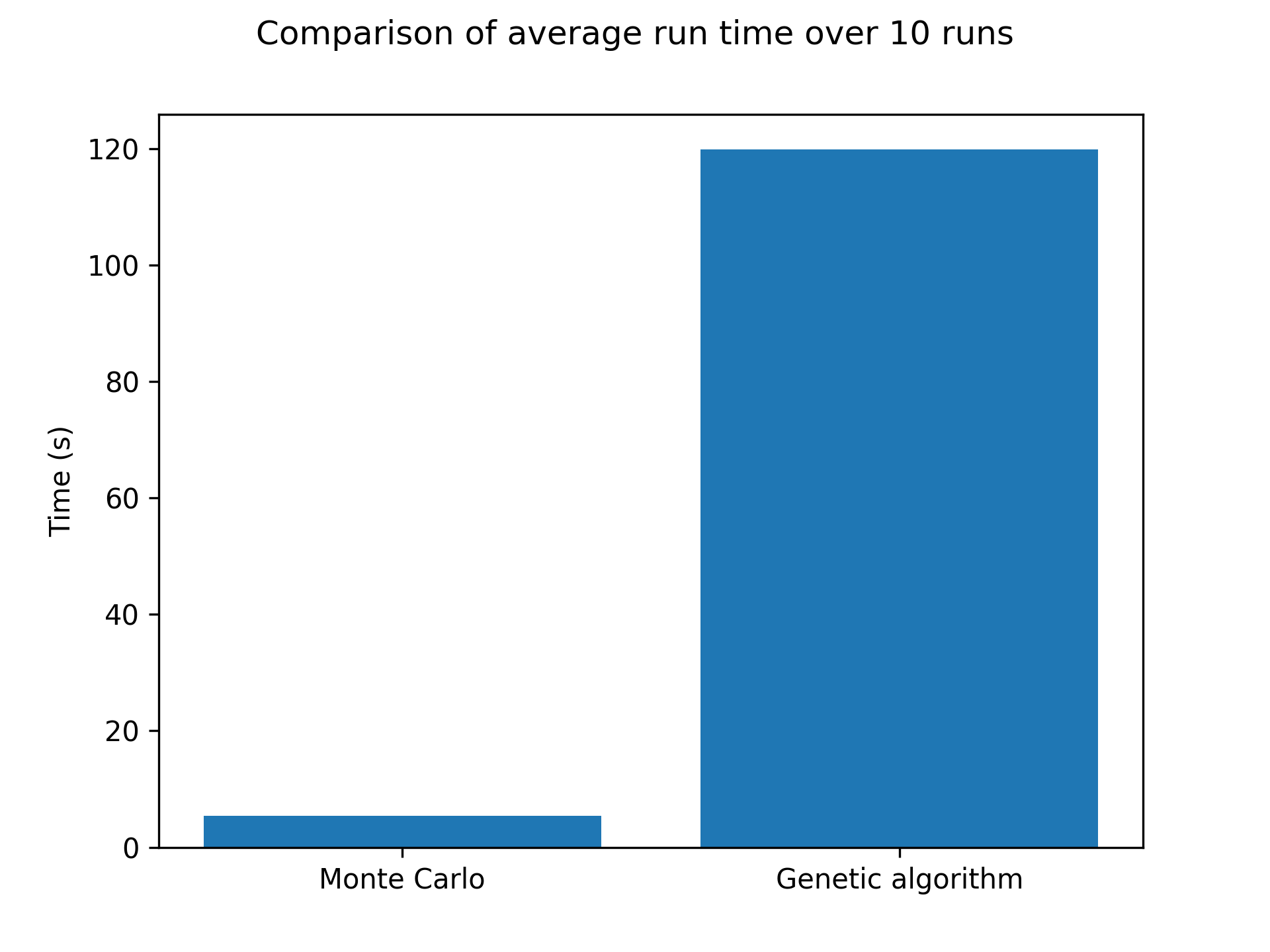
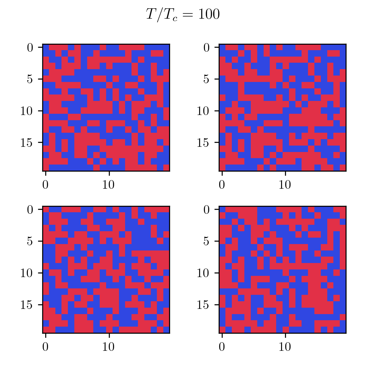
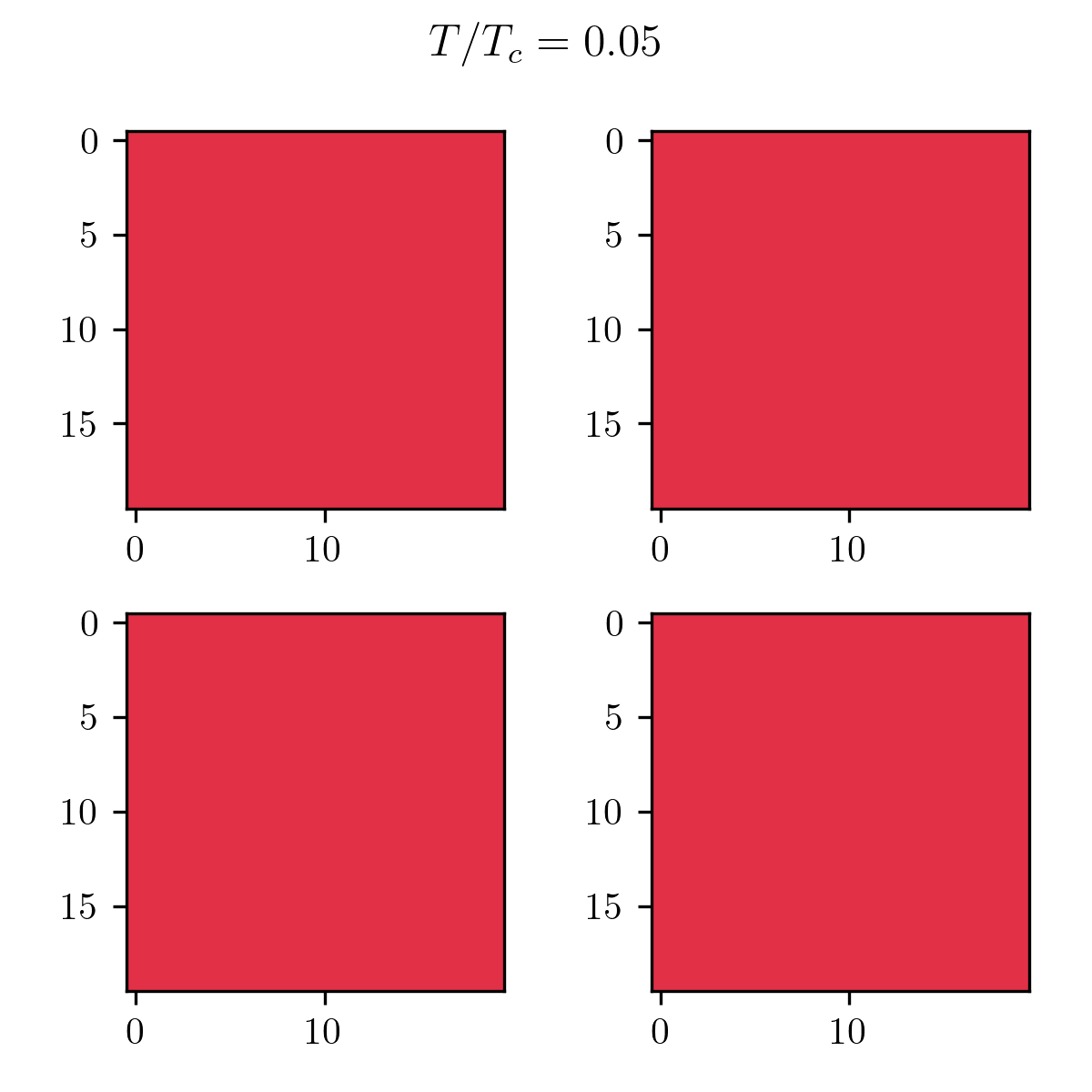
Comparison of average run time over 50 runs

As you can see, it’s pretty bad! In terms of results, just like the Monte Carlo algorithm, after enough generations the population will represent the correct temperature equilibrium. You can see that in the following pictures showcasing the four fittest members of the final population at low and high temperatures.

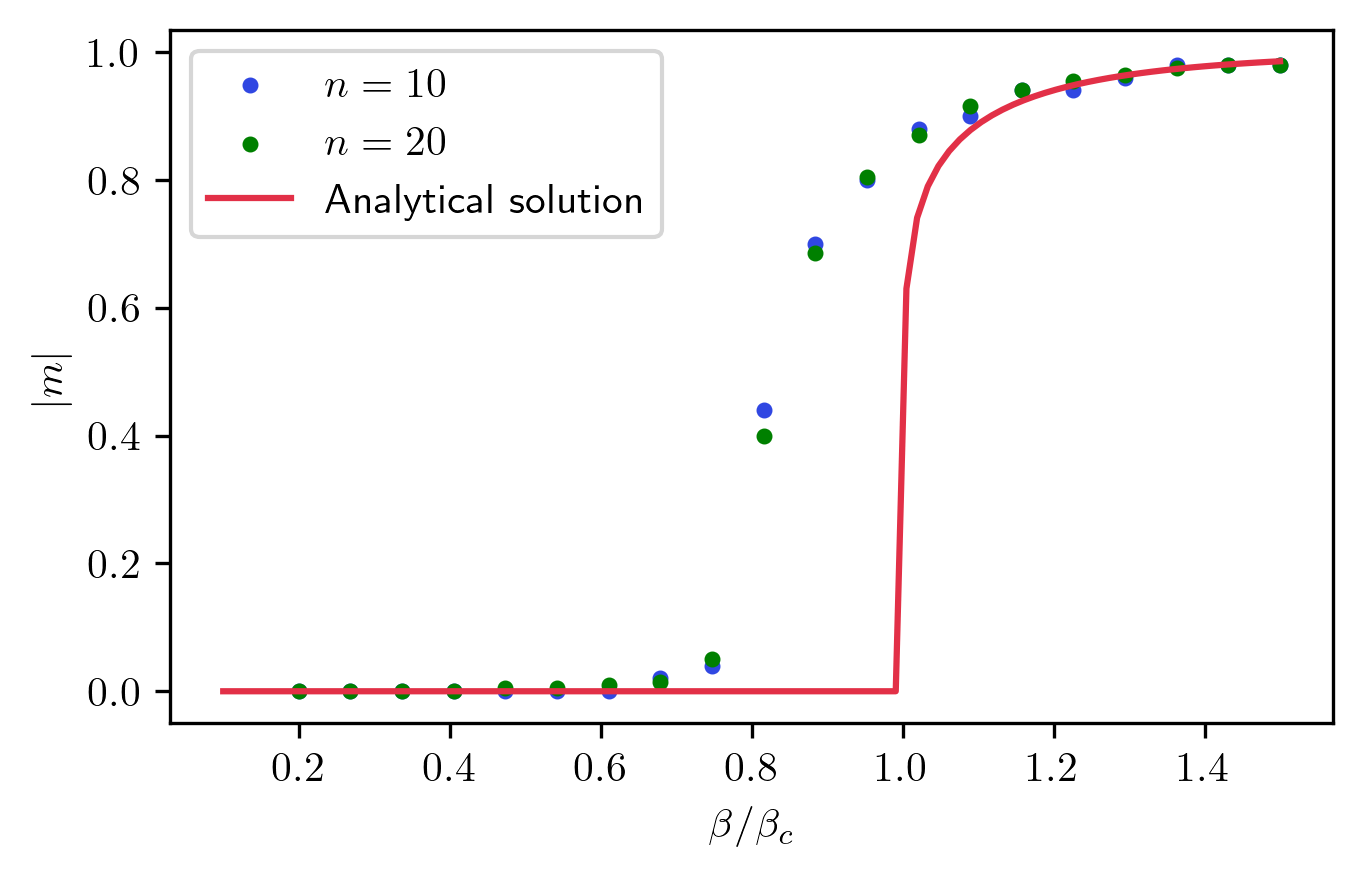
Finally, I can compare the magnetization to the exact solution to see how this algorithm fares near the transition. From this picture, you can see that this method gives a good approximation of the magnetization curve, with one caveat. The transition seems slightly shifted to lower temperatures. This is simply an effect of the approximation made to compute the entropy. ⁴

Genetic magnetization vs exact solution

Final remarks

Well, this has been quite a tour of the Ising model! I’ve explored two different approaches to solving this classic problem in statistical physics: the tried-and-true Monte Carlo method with Metropolis sampling, and the more creative approach using genetic algorithms. The goal here was really to have some fun with genetic algorithms in a setup that I was familiar with, like the Ising model.

The genetic algorithm approach, while not quite as accurate or efficient as the Monte Carlo method, showed that optimization methods can be of great help to solve complex physics problems! Now, you might be wondering, why bother with genetic algorithms if Monte Carlo works better? Genetic algorithms shine in optimization problems, especially when the solution space is vast and complex. In this case, I used it to minimize the free energy of the system—a task that becomes increasingly challenging as models become more and more complex. Perhaps other interesting optimization methods, such as particle swarm optimization, can similarly be of some use to physicists who are not aware of them.

So, whether you’re a seasoned researcher or an enthusiastic amateur, I hope this exploration has sparked your curiosity and inspired you to delve deeper into the world of computational physics. Till next time!

NOTE

All the code for this project can be found on this Github repository.

Footnotes

Ising, E. Beitrag zur Theorie des Ferromagnetismus. Z. Physik 31, 253–258 (1925). (In German) ↩
Onsager, L. Crystal Statistics. I. A Two-Dimensional Model with an Order-Disorder Transition. Phys. Rev. 65, 117 (1944). ↩
T. Bacerzak, Thermodynamics of the Ising model in pair approximation. Physica A: Statistical Mechanics and its Applications, Vol. 317, No 1–2, pp 213-226 (2003). ↩
T. Gwizdalla, The Ising model studied using evolutionary approach. Modern Physics Letters B, Vol. 19, No. 04, pp. 169-179 (2005). ↩ ↩² ↩³