Physics informed neural networks

PINN: how do they work?

Neural networks (NNs) are fundamentally a great way to approximate complicated continuous functions of many variables. The building blocks of NNs are simple:

• linear operations $x_i \to a_{ij} x_j + b_i$,
• smooth non-linear functions such as the hyperbolic tangent or the sigmoid function.

When composing these operations, you make a neuron. By connecting stacks of these neurons together in layers, it is possible to get extremely complex output. All that’s left is tuning all the parameters $a_{ij}, b_i$ for each neuron in each layer. These quickly grow in size: for a simple (1, 64, 128, 64, 1) dense neural network (where each number indicates the number of neurons in each layer), you have to tune more than 16k parameters.

This step is called training the network, where the network is fed some input and returns some numbers as output, which are compared to some reference output (usually, those are labels of the ground truth). The parameters are then all slightly tuned to make this output closer to whatever reference value we have. Through this process, we are exploring the parameter landscape and looking for a global minimum of our loss function, usually by using some derivative of the gradient descent algorithm. After doing this enough times, one hopes that the trained network output approximates the distribution of the training data as well as generalizes to any new example.

The main idea behind PINNs is to use this property of the NNs as universal continuous function approximators to learn the solution to the differential equation of interest. Instead of evaluating the loss of the output of the NN compared to some labels, we assume that the output should solve the differential equation itself (up to some parametrization choice) and so we use the differential equation as a loss function. The process is then more or less the same, except you feed the NN with different points of your domain, then plug the output inside the differential equation and use the residual to tune the parameters closer to an optimum. Importantly, unlike in supervised learning, there is no need to curate a training dataset here, you just keep evaluating your model on randomly sampled points in the domain you’re interested in.

One important caveat of this method is boundary conditions: when you solve a differential equation $\mathcal M[y] = 0$, you also need to provide enough boundary conditions (values and derivatives for an initial-value problem, values at boundaries for a boundary-value problem) to uniquely determine the solution. There are two ways to do this:

• you can add the constraints as penalty terms on the loss function, so the optimization process fixes both the solution and its boundary conditions,
• or, you can parametrize the solution (what we usually call in physics an ansatz) in such a way that the conditions are automatically applied.

In the first case, you just define the loss function on your output $y$ as

where in practice, each term can and should be weighted differently. This method is equivalent to “adding up” all the sources of errors and minimizing them all at the same time. In the examples below, I will be using a package which relies on this method by default. To give an example of the second method, consider the following initial-value problem

I mentioned previously that PINNs model the solution to the equation from the output $N(t)$ of the neural network. However, you can also use that output as a building block for a more complex function. In the case I just presented, the parametrization

automatically satisfies the initial value conditions⁵. So instead of training the network so that $N$ is a solution to the equation, you can train the network so that $y$ is a solution. That way, you get the initial value conditions for free and the network will simply adapt.

Okay, so why are these models useful?

The main advantage of PINNs is that they provide mesh-free solutions to differential equations. Usually, to solve this kind of problem, you need to discretize the space on which the solution exists (the mesh), and then you can for example approximate the derivatives of the solution by the values at nearby points, so that your problem becomes algebraic and amenable to all sorts of numerical methods. With a PINN, you can use the autograd properties of your favorite tensor package to calculate the loss function at much greater accuracy, and in particular it doesn’t depend on the size of the mesh you use to train the model. Moreover, these methods tend to require much fewer points to approximate the solution than mesh-based methods do (I will showcase this in the examples below). The mesh-free nature of these methods also comes in handy when dealing with unusual geometries: you can just sample random points inside the geometry instead of having to create a special, complex mesh. This is very useful in areas like fluid dynamics where you might have a custom geometry for your problem.

Another interesting advantage of these methods is how trendy deep learning methods are. There is currently a lot of money and efforts directed towards improving NN training efficiency, both on a technical level as well as on a hardware level (GPUs, TPUs). Any such improvement is bound to spill out to any other application, including PINNs!

Examples

Let’s now take a look at various examples of differential equations matching real physical systems. To solve these, I am using the DeepXDE library which abstracts away a lot of the difficulties and intricacies you might encounter. However, if you are interested in learning more about the nitty gritty of PINNs, I highly recommend implementing your own architecture from scratch for at least one example.

Simple harmonic oscillator

Theory

When working with new ideas and methods, it’s always good to start with a simple model for which you already know the answer. The typical model for this in physics is the harmonic oscillator (think a mass on a spring moving back and forth). This model has far-reaching importance throughout all of physics: at a simplified level, it describes systems such as sound waves in metals or electrical RLC circuits, while its quantum counterpart is at the root of the quantized energy description of atoms. The dynamics of the harmonic oscillator are governed by the following differential equation:

$$\partial_t^2 y + \xi \omega_0 \, \partial_t y + \frac{\omega_0^2}{4} y = 0~.$$

In this equation, $\omega_0$ is a proper frequency of the system, and $\xi \omega_0$ accounts for fluid friction (due to air resistance for example). In the rest of this example, I will only be interested in solutions satisfying the initial value constraints $y(t=0) = 1$ and $y^\prime(t=0) = 0$; back to the spring analogy, this would mean starting the system with the spring extended by 1 unit, and releasing it delicately.

This system admits two types of solutions: when $\xi_0 \neq 1$, the solution takes the form $c_0 e^{-\omega_+ t} + c_1 e^{-\omega_- t}$ where $\omega_\pm$ are the roots of the associated second order polynomial:

$$\omega_\pm \equiv \xi \pm \omega = \frac{\xi_0 \omega_0}{2} \pm \frac{\omega_0 \sqrt{\xi_0^2 - 1}}{2}~.$$

For my choice of initial values, the solution simplifies to

$$y(t) = e^{- \xi t} \Bigl[ y_0 \cos(\omega t) + \frac{y_1 + \xi y_0}{\omega} \sin(\omega t) \Bigr]~.$$

Note that for $\xi > 1$, $\omega$ becomes purely imaginary and the cosine and sine turn into their hyperbolic counterparts. There is another case to consider: when $\xi_0 = 1$, the two branches are degenerate and the general (or critical) solution becomes

$$y(t) = e^{- \xi t} \Bigl[ y_0 + (y_1 + \xi y_0) t \Bigr]~.$$

Setup

Now that we’ve clarified the math a bit, let’s move to solving the problem. To start with, initialize your virtual environment with whatever tool you prefer⁶ and with the following dependencies:

# pyproject.toml
[project]
requires-python = "==3.12"
dependencies = [
    "deepxde==1.13.1",
    "torch==2.6.0",
]

First we are going to define a class specifying the details of the harmonic oscillator system:

class HarmonicOscillator0D:
    """Class modeling the harmonic oscillator in 0+1 dimensions. The ODE is:
    $$
        \\frac{\\partial^2 y}{\\partial t^2} + \\xi_0 * \\omega_0 * \\frac{\\partial y}{\\partial t} + \\frac{\\omega_0^2}{4} y = 0
    $$
    and with initial conditions $y(t = 0) = y_0, y^\\prime(t = 0) = y_1$.


    Args:
        omega0 (float): Intrinsic frequency of the system.
        xi0 (float): Fluid friction term.
        y0 (float): Initial value of the solution.
        y1 (float): Initial derivative of the solution.
    """

    __slots__ = ("xi0", "omega0", "xi", "omega", "y0", "y1")

    def __init__(self, xi0: float, omega0: float, y0: float, y1: float):
        # ODE parameters
        self.xi0 = xi0
        self.omega0 = omega0
        self.xi = xi0 * omega0 / 2
        self.omega = self.omega0 * np.sqrt(np.abs(np.power(self.xi0, 2) - 1)) / 2

        # Initial value condition
        self.y0 = y0
        self.y1 = y1


    def equation(self, x: torch.Tensor, y: torch.Tensor) -> torch.Tensor:
        """Defines the ODE.

        Args:
            x (torch.Tensor): Input of the neural network.
            y (torch.Tensor): Output of the neural network.

        Returns:
            (torch.Tensor): Residual of the differential equation.

        """
        pass

    def initial_value(self, x: torch.Tensor) -> torch.Tensor:
        """Defines the initial value for the differential equation.

        Args:
            x (torch.Tensor): Input of the neural network.

        Returns:
            (torch.Tensor): Value at the boundary for the initial condition.
        """
        pass

    def initial_value_derivative(
        self, x: torch.Tensor, y: torch.Tensor, X: np.ndarray
    ) -> torch.Tensor:
        """Defines the initial value of the derivative for the differential equation.

        Args:
            x (torch.Tensor): Input of the neural network.
            y (torch.Tensor): Output of the neural network.
            X (np.ndarray): Numpy array of the inputs.

        Returns:
            (torch.Tensor): Residual of the initial value condition for the derivative.
        """
        pass

    def exact_solution(self, x: np.ndarray) -> np.ndarray:
        """Defines the ground truth solution for the system.

        Args:
            x (np.ndarray): Points on which to evaluate the solution.

        Returns:
            (np.ndarray): Value of the solution on the points.
        """

        pass

For this example, I will detail each function step by step before moving on the code to solve the problem. The method exact_solution encodes the ground truth, the analytical solution I derived previously, and I will use this function to test my neural network architecture:

def exact_solution(self, x: np.ndarray) -> np.ndarray:
    # Damping term
    exp_term = np.exp(-self.xi * x)
    # Critical case
    if self.xi0 == 1:
        c0 = self.y0
        c1 = self.y1 + self.xi * self.y0
        return exp_term * (c0 + c1 * x)
    else:
        c0 = self.y0
        c1 = (self.y1 + self.xi * self.y0) / self.omega
        # Underdamped case
        if self.xi0 < 1:
            return exp_term * (
                c0 * np.cos(self.omega * x) + c1 * np.sin(self.omega * x)
            )
        # Overdamped case
        else:
            return exp_term * (
                c0 * np.cosh(self.omega * x) + c1 * np.sinh(self.omega * x)
            )

The class also features two methods which will be used to fix the two initial value condition. By now you might have already noticed that the two methods have different signatures and impose each initial value condition differently. This comes down to how DeepXDE will impose the initial value condition.⁷ For the Dirichlet condition, you just need to return the value at the $t = 0$ slice,

def initial_value(self, x: torch.Tensor) -> torch.Tensor:
    return y0

while for the Neumann condition, the function returns the difference between the derivative and the value we are aiming for

def initial_value_derivative(
    self, x: torch.Tensor, y: torch.Tensor, X: np.ndarray
) -> torch.Tensor:
    dy_dt = cast(torch.Tensor, dde.grad.jacobian(y, x, i=0, j=0))
    return dy_dt - self.y1

Finally, the equation of motion inside the domain is imposed via the equation method

def equation(self, x: torch.Tensor, y: torch.Tensor) -> torch.Tensor:
    dy_dt = cast(torch.Tensor, dde.grad.jacobian(y, x, i=0, j=0))
    dy2_dt2 = cast(torch.Tensor, dde.grad.hessian(y, x, i=0, j=0))
    ode = dy2_dt2 + self.xi0 * self.omega0 * dy_dt + (self.omega0**2 / 4) * y
    return ode

One of the greatest perks of the DeepXDE library is that it caches the gradient calculations. The interface to calculate the Jacobian and Hessian components is therefore simple yet performant!

Now we can use this class to solve the problem for various values of the parameters. Let’s start by setting up some constants

xi0 = 0.1
omega0 = 2 * np.pi * 5
y0 = 1
y1 = 0

# Neural network parameters
input_size = [1] 
output_size = [1] 
layers_sizes = input_size + [64, 128, 64] + output_size
activation = "tanh"
initializer = "Glorot normal"

# Training parameters
optimizer_kw = dict(
    lr=0.001,
    metrics=["l2 relative error"],
    loss_weights=[0.001, 1, 0.5],
)
n_iterations = 10_000

# Mesh parameters
n_training_inside = 64
n_training_bdy = 2
n_test = 500

Most of these are easy to understand from their names: the neural network’s architecture will be composed of dense layers (the number of units is specified by layers_sizes and will be initialized using the Xavier normal initializer) and $\tanh$ activation functions. The network will be trained over 10,000 iterations, using 64 random points inside the domain and testing the output against the exact solution on 500 points. An important hyperparameter to tweak for this kind of model is the list of weights loss_weights of the loss function terms (interior ODE loss, Dirichlet initial value loss, Neumann initial value loss). When training the model, if you see that one of these losses stagnate compared to others, increasing its relative weight is a great way to boost the learning process.

When using DeepXDE to solve a problem like this one, you must then follow 4 different steps:

1. define the domain on which to solve the problem,
2. define the boundary or initial value conditions (and associated boundary slices selectors),
3. generate the training and testing data,
4. initialize and train the model.

For this problem, the code for these steps is

# 1. Define the domain
geom = dde.geometry.TimeDomain(0, 1)

# 2.0 Create the harmonic oscillator object
ho = HarmonicOscillator0D(xi0=xi0, omega0=omega0, y0=y0, y1=y1)
# 2.1 Define the t=0 slice boundary
def boundary_t0(x: torch.Tensor, on_boundary: bool) -> bool:
    return on_boundary and dde.utils.isclose(x[0], 0)
# 2.2 Define the initial value conditions
ic_value = dde.icbc.IC(geom, ho.initial_value, lambda _, on_initial: on_initial) # The on_initial boolean defines the t = 0 slice.
ic_derivative_value = dde.icbc.OperatorBC(
    geom, ho.initial_value_derivative, boundary_t0
)

# 3. Generate the training and testing data
data = dde.data.TimePDE(
    geom,
    ho.equation,
    [ic_value, ic_derivative_value],
    num_domain=n_training_inside,
    num_boundary=n_training_bdy,
    solution=ho.exact_solution,
    num_test=n_test,
)

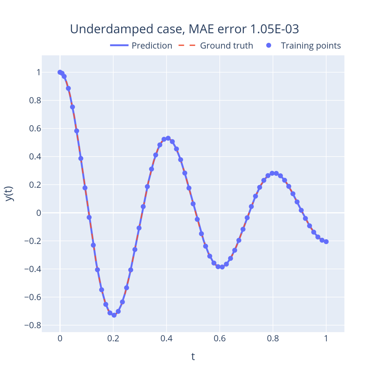
# 4.1 Initialize the model
neural_net = dde.nn.FNN(layers_sizes, activation, initializer)
model = dde.Model(data, neural_net)
model.compile("adam", **optimizer_kw)
# 4.2 Train the model
losshistory, train_state = model.train(iterations=n_iterations)

Now let’s look at some results! I ran the above code for multiple values of $\xi_0$. First, the simple case without friction ($\xi_0 = 0$) where the mass keeps oscillating back and forth. When you tune the friction coefficient up, the oscillations start to weaken with time (this is called the underdamped regime).

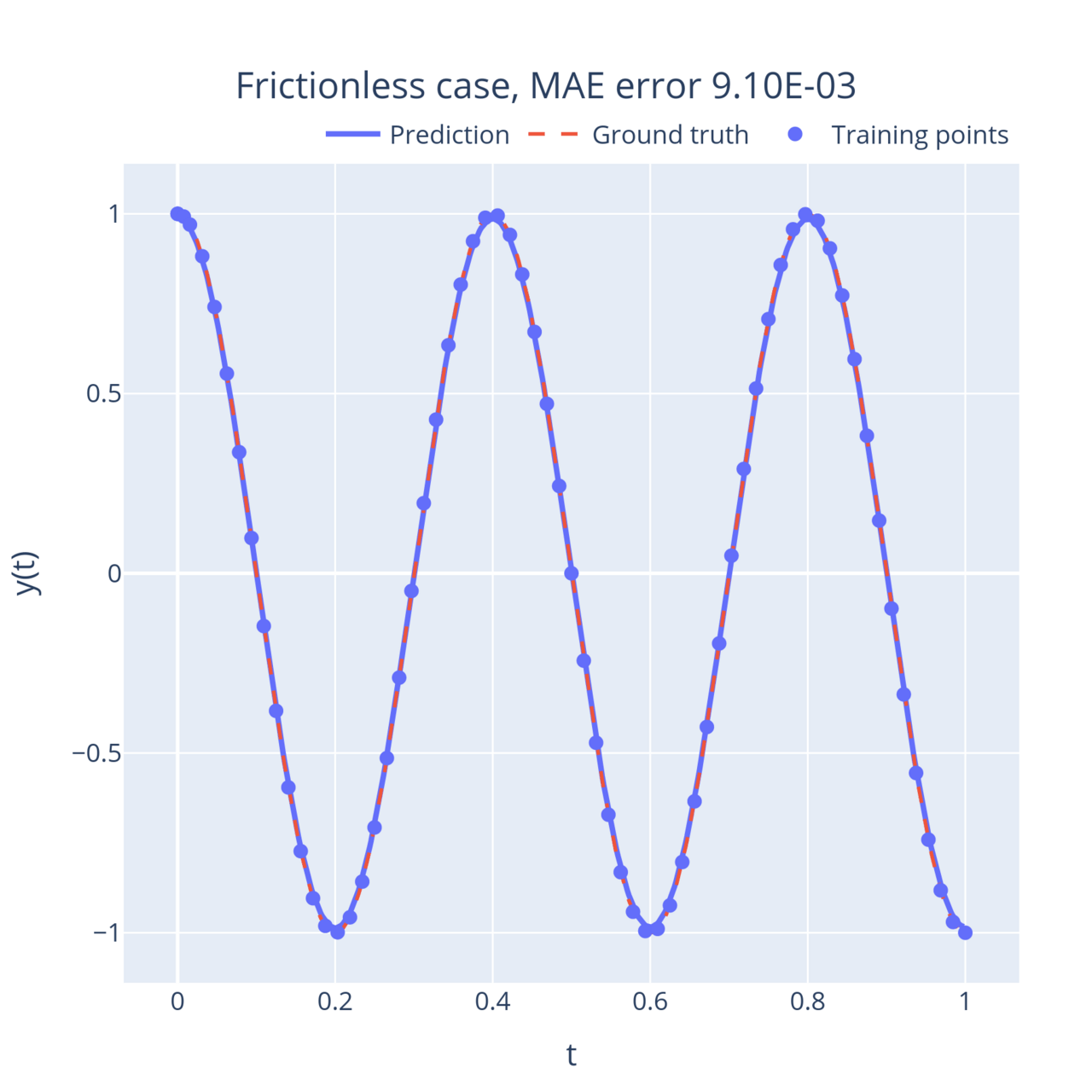
On the other end of the spectrum, when the friction coefficient is large, the mass returns to its stable position exponentially instead of oscillating (this is called the overdamped regime). Interestingly, this movement slows down as the friction term increases. In between, when $\xi_0 = 1$, the system reaches a critical point (the degenerate solution derived above). This point is the fastest the system can return to its equilibrium without oscillating:

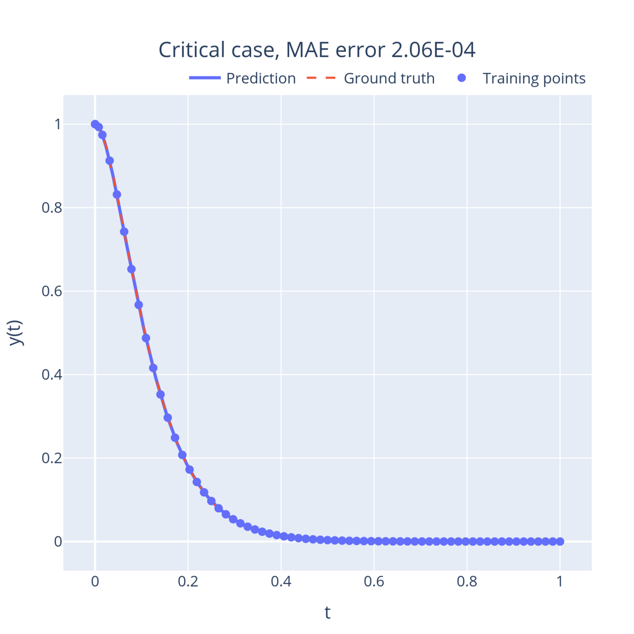
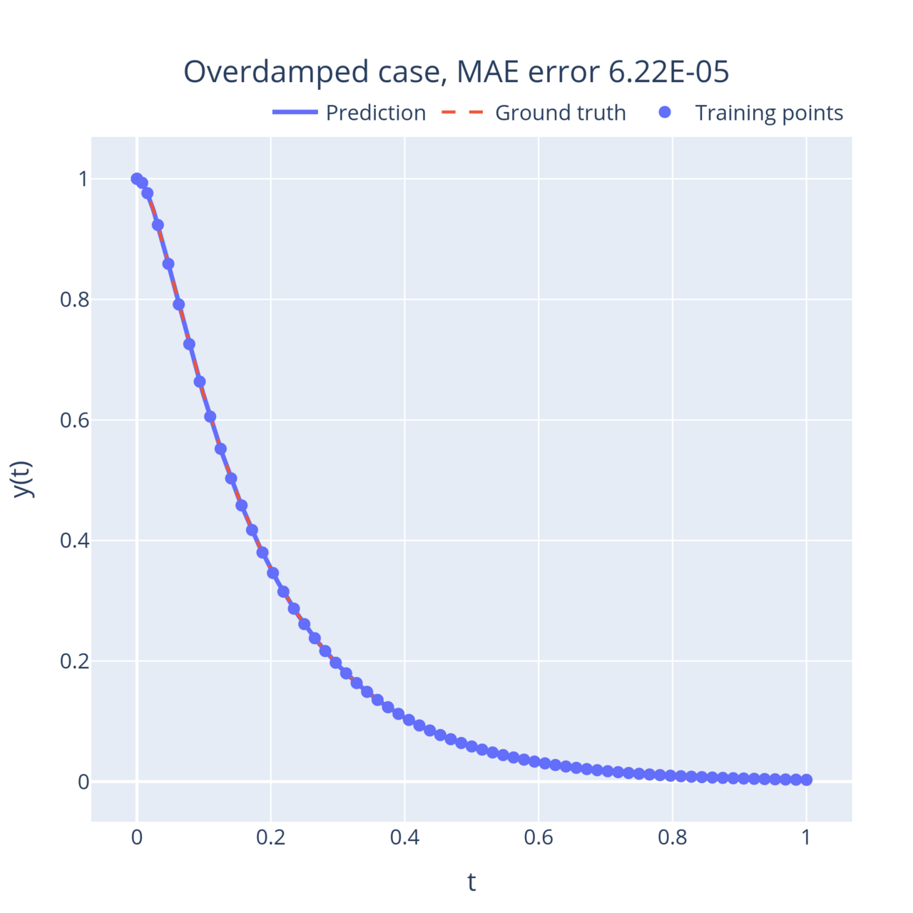
In all these examples, the neural network learnt to approximate the solution to the equations with very few training points, and can then output an accurate solution anywhere in the domain.

Heat equation

Okay let’s ramp up the difficulty a little bit! The heat equation which describes the diffusion of temperature in a medium is another classical example. To put it in concrete terms, imagine you take a needle, and heat it. After you stop, the electrons inside the needle will bounce off each other, spreading the energy (and therefore the heat), until the temperature of the needle is the same everywhere. This process is called energy diffusion and is described by the following equation:

$$\partial_t T(t,x) = \kappa \partial_x^2 T(t,x)~,$$

where $\kappa$, called the thermal diffusivity, quantifies how fast the heat spreads. I need to choose some boundary conditions and initial value profile before I can solve this: in this example I took $T(t=0, x) = \sin(n \pi x)$ (with $n \geq 1$ an integer) and $T(t, x=0) = 0$ and $T(t, x=1) = 0$. The analytical solution can be obtained easily⁸ and takes the form of an exponential decay of the initial temperature profile:

$$T(t,x) = \sin(n \pi x) e^{- n^2 \pi^2 t}~.$$

At this point you might be worried that $T$ can become negative (for example when $1 < x < 2$ and $n=1$). The reason for this is that this equation does not apply to the absolute temperature of the system, but its temperature relative to a baseline. The initial profile we apply is periodic with some pockets above and some below the baseline, and as time progresses that temperature profile diffuses until the temperature is constant everywhere, and therefore the relative temperature is zero.

To solve the equation numerically using DeepXDE, you can use pretty much the same setup with the following differences:

• the input layer of the neural network should be two-dimensional instead of one-dimensional since there are now two coordinates,
• the model should now be given an initial profile on the entire $t=0$ slice as well as Dirichlet boundary conditions at both $x=0$ and $x=1$,

bc = dde.icbc.DirichletBC(
    geom_full, lambda x: 0, lambda _, on_boundary: on_boundary
)
ic = dde.icbc.IC(
    geom_full,
    lambda x: np.sin(n * np.pi * x[:, 0:1]),
    lambda _, on_initial: on_initial,
)

• the model should be trained with samples on both the boundary and initial value slice

n_training_inside = 2000
n_training_bdy = 80
n_training_initial = 160
n_test = 2000

data = dde.data.TimePDE(
    geom_full,
    heat_eq.equation,
    [bc, ic],
    num_domain=n_training_inside,
    num_boundary=n_training_bdy,
    num_initial=n_training_initial,
    solution=heat_eq.exact_solution,
    num_test=n_test,
)

where heat_eq is the equivalent to the HarmonicOscillator0D object from before, but adapted to this system. After training the model for both $n=1$ and $n=4$ and with $\kappa = 0.1$, these are the results:

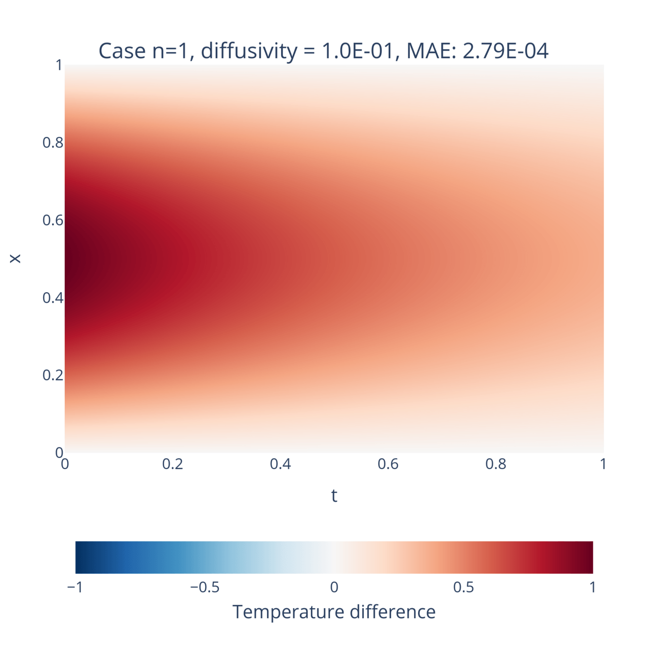
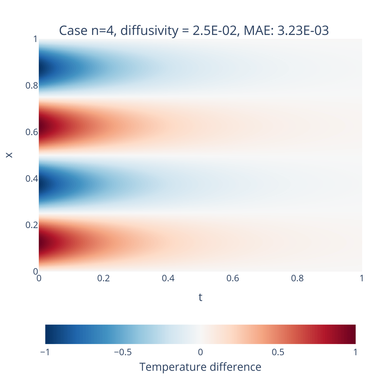
Hurray! Once again the neural networks has correctly learnt the solution to the equations and generalizes quite well beyond the training data. For reference, the network was trained on a little bit more than 2000 points, while the mesh of the figures consist of 1 million points. This is a great example of the natural interpolation property of PINNs!

Summary

In this post, I wanted to give you brief introduction to PINNs as well as show how neural networks and deep learning in general can have great application in numerical physics. In the examples I derived, you can clearly see the quality of solutions they yield. However most of these examples are rather simple, mostly due to resource constraints (I just don’t have a great GPU laying around), and this method is currently more resource-hungry than traditional finite-element methods. On the other end, its ability to naturally capture unusual geometries is very promising.